If you’ve been using Google Sheets and find yourself frequently searching for specific data, you’ll be glad to learn about the MATCH Function in Google Sheets . It’s a powerful tool that helps you quickly locate the position of a specific value within a range. But what makes it so special? Let’s dive into the details!
Why Should You Use the MATCH Function in Google Sheets?
Imagine you have a large dataset, and you want to know the position of a particular value within a column. Doing this manually could take forever, but with MATCH, you can find the exact row or position in just a few seconds. The best part? It works perfectly with other Google Sheets functions like VLOOKUP and INDEX, making it incredibly versatile.
In this post, we’ll walk through a real-world example to show how to use this function effectively.
Example Dataset
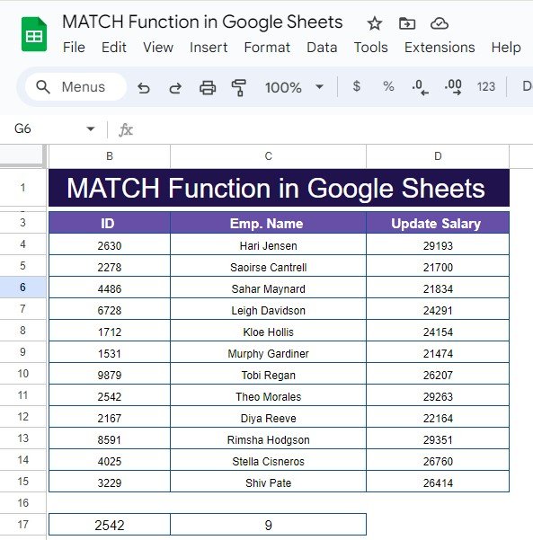
Let’s start with some sample data. We have a list of employees along with their ID numbers and updated salary figures. The data is arranged in B3
in your Google Sheets: Now, let’s say you want to find out the row number where Theo Morales’s employee ID (2542) is located.

Applying the MATCH Function
To do this, we’ll use the MATCH function. The formula we’ll use is:
=MATCH(B17,B3:B15,0)
Breaking Down the Formula:
- B17: This is where you input the value you’re searching for—in this case, it’s employee ID 2542.
- B3: This is the range where Google Sheets will look for that employee ID.
- 0: The final argument tells the function to look for an exact match.
When you run this formula, Google Sheets will search the range B3
and return the position of the employee ID 2542.
What’s the Output?
After applying the formula, the result is:
This means that the employee ID 2542 (Theo Morales) is located in the 9th row of the given range.

Why Use MATCH? Here Are Some Key Benefits
- Time-Saving: Instead of scrolling through a large dataset manually, you can instantly find the position of any value within a range.
- Versatile: MATCH is often used in combination with other functions like VLOOKUP or INDEX to create dynamic formulas that adapt to your data.
- Precise: By specifying an exact match (as we did with the 0 in the formula), you avoid potential errors in your data search.
Final Thoughts
The MATCH function is a simple but powerful tool that can save you tons of time when working with large datasets in Google Sheets. Whether you’re searching for an employee ID or any other value, this function will quickly help you pinpoint its location.
Visit our YouTube channel to learn step-by-step video tutorials
Youtube.com/@NeotechNavigators
View this post on Instagram