If you’ve ever wondered how to quickly calculate mileage reimbursement using Google Sheets, you’re in the right place! In this post, we’ll walk you through an easy formula that simplifies the entire process, allowing you to track miles driven, reimbursement rates, and calculate your total payouts accurately. Whether you are managing a business budget or personal expenses, this formula is your best friend.
Let’s dive into it step-by-step with a real-life example!
Data Setup: What You’ll Need
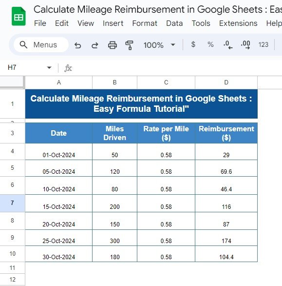
Before applying the formula, let’s get the data ready. In our example, we are working with the following data arranged in Google Sheets from cell A3 to D10. The key data points include:
- Date: The day the mileage was recorded.
- Miles Driven: The total miles driven on that specific day.
- Rate per Mile ($): The reimbursement rate per mile driven.
- Reimbursement ($): The total amount to be reimbursed, which we’ll calculate using our formula.
Below is what the data looks like:
The Formula: Calculate Mileage Reimbursement Easily
To calculate the reimbursement amount for each entry, we’ll use a simple multiplication formula in Google Sheets. All you need to do is multiply the miles driven by the rate per mile.
Here’s the formula we’ll use:
=B4*C4
Let’s break it down:
B4 refers to the miles driven on a specific day.
C4 refers to the reimbursement rate per mile.
The formula multiplies these two values to calculate the total reimbursement for each day.
Example Calculation:
For the first row: This same formula applies to all the rows by simply dragging the formula down through the column.
Output: Calculate Mileage Reimbursement in Action
After applying the formula to all rows, here is the final result:
Using Auto-fill for Faster Results
To save time, Google Sheets allows you to auto-fill the formula across rows. Just follow these steps:
Enter the formula in the first row (for example, in cell D4).
Click on the bottom-right corner of the cell (you’ll see a small blue square).
Drag the formula down to apply it to all relevant rows.
This way, all the calculations will be done automatically for every entry!
Why This Formula is So Helpful
- Time-saving: Automates the reimbursement calculation across multiple entries.
- Accurate: Ensures that no manual mistakes occur during reimbursement tracking.
- Simple: Easy enough for beginners and perfect for small business or personal use.
Pro Tip: Customize for Variable Rates
If the reimbursement rate varies across different trips, no worries! Simply modify the values in the “Rate per Mile” column, and the formula will adjust accordingly. This flexibility makes it ideal for tracking fluctuating rates.
Conclusion: Mileage Reimbursement Made Easy
Using this straightforward formula in Google Sheets, calculating mileage reimbursement is fast, efficient, and error-free. Whether you’re handling reimbursements for personal expenses or managing them for a business, this method simplifies the entire process. Plus, Google Sheets allows easy tracking and updates, making it your perfect tool for managing mileage-based reimbursements.
Visit our YouTube channel to learn step-by-step video tutorials
Youtube.com/@NeotechNavigators

