Are you looking to rank data based on percentiles but aren’t sure where to start? Don’t worry! In this blog post, I’ll guide you through how to use the PERCENTRANK function to rank your data effectively and easily. Whether you’re analyzing student scores, sales data, or any other type of data, PERCENTRANK is a handy function that helps you understand where each data point stands in relation to others.
Let’s jump in and explore how to use this function with a clear example!
What Is the PERCENTRANK Function?
First things first, what does the PERCENTRANK function do? Well, it ranks each value in a dataset by showing where it falls on a percentile scale of 0 to 1. This is super helpful when you want to see how each value compares to the rest.
The formula for the PERCENTRANK function looks like this:
=PERCENTRANK(array, x)
Here’s what each part means:
- Array: This is the range of data you’re ranking (e.g., scores).
- X: This is the specific value you want to rank within the dataset.
In simpler terms, PERCENTRANK tells you the percentage of data points that are less than or equal to the value you’re ranking. If a student’s score ranks at 0.765, for instance, that means 76.5% of the other scores are below or equal to that student’s score.
Step-by-Step Example: Rank Student Scores Using PERCENTRANK
Now that you have a basic understanding of how PERCENTRANK works, let’s dive into a practical example. We have a dataset of student scores, and we’ll use the PERCENTRANK function to rank each student based on their score.
Here’s the data we’ll be working with:
Step 1: Set Up Your Data in Excel
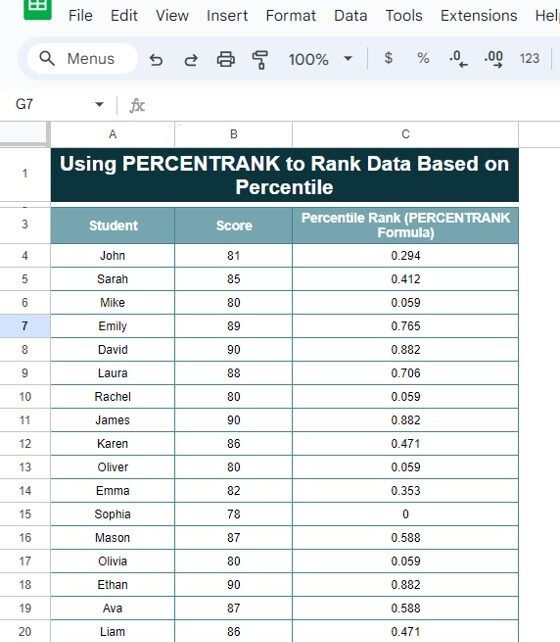
To get started, open your Excel sheet and enter your data. In this example, we have Student Names in column A, Scores in column B, and we’ll calculate the Percentile Rank in column C using the PERCENTRANK function.
Your data should look something like this:

Step 2: Apply the PERCENTRANK Formula
Now, let’s calculate the percentile rank for each student. In Cell C4, enter the following formula:
=PERCENTRANK($B$4:$B$21, B4)
Here’s what this formula does:
$B$4:$B$21 is the range of all student scores.
B4 is the score of the first student (John in this case), which we are ranking.
Step 3: Drag the Formula for Other Students
Once you’ve entered the formula for the first student, you don’t need to manually calculate the rank for each student. Simply drag the formula down for the rest of the rows. Excel will automatically update the formula for each student and rank them based on their score.
Understanding the Output
After applying the formula, you’ll see the results in the Percentile Rank column. For example:
John with a score of 81 is ranked at 0.294.
David with a score of 90 is ranked at 0.882.
Sophia with a score of 78 is ranked at 0, meaning her score is the lowest in the dataset.
The higher the percentile rank, the better the student performed relative to others. A student ranked at 0.882 has a score that’s higher than 88.2% of the other students.

Why Use PERCENTRANK?
There are several reasons why PERCENTRANK is a valuable function:
- Helps compare performance: You can easily see how one value stacks up against the rest of the dataset.
- Works with any type of data: Whether you’re working with test scores, sales data, or financial numbers, PERCENTRANK helps you understand data distribution.
- Simple to use: Once you’ve set up the formula, it’s just a matter of dragging it down to rank your entire dataset.
Final Output
Here’s a snapshot of what the final output will look like:
Conclusion
And there you have it! Using the PERCENTRANK function in Excel is a simple yet powerful way to rank data based on percentile. Whether you’re ranking student scores or other datasets, PERCENTRANK gives you a clear understanding of how each value compares to the rest. Try it out with your own data and see how easy it is to use!
Visit our YouTube channel to learn step-by-step video tutorials
Youtube.com/@NeotechNavigators
View this post on Instagram
Click here to Make the copy of this Template