If you’ve ever needed to find the minimum value in a dataset based on specific criteria, the MINIFS function in Google Sheets is here to make your life easier! Whether you’re analyzing sales data, project progress, or any other type of information, this function can help you quickly get the results you need. In this post, I’ll walk you through exactly how to use the MINIFS function in Google Sheets with a real-life example.
What is the MINIFS Function in Google Sheets?
Before we get into the details, let’s talk about what the MINIFS function does. Essentially, this function helps you find the minimum value in a range based on one or more criteria. In other words, if you want to find the lowest number that matches certain conditions—like the smallest sale made in a specific city—the MINIFS function can do that for you in just one step.
Sounds great, right? Now, let’s look at how it works with an example!
Example Data: Finding the Minimum Sale Based on City
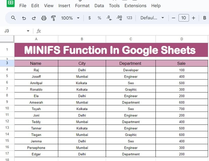
For this example, we’ll be using a dataset that contains sales data for different departments across multiple cities. Here’s what our data looks like:
Now, let’s say we want to find the minimum sale in Delhi. This is where the MINIFS function comes in handy.

Step-by-Step Guide: How to Use the MINIFS Function
Here’s how you can apply the MINIFS function to get the minimum sale in a specific city like Delhi.
First, select the cell where you want to display the result. For this example, we’ll use cell A19 for our criteria (the city we want to search by, which is “Delhi”).
Next, enter the formula in the cell where you want to show the result. The formula we’ll use is:
=MINIFS(D4:D17,B4:B17,A19)
Let’s break this down:
D4is the range that contains the sales data (the numbers we want to find the minimum of).B4
is the range where the city names are listed.
A19 is the cell that holds our criteria (in this case, “Delhi”).
Hit Enter, and you’ll instantly see the result—Google Sheets will return the smallest sale made in Delhi.
Breaking Down the Formula
Let’s take a closer look at what’s happening with this formula:
- MINIFS: This is the main function that finds the minimum value based on the criteria you set.
- D4: This is the range that contains the values you want to evaluate (in our case, sales amounts).
- B4: This is the criteria range—in this example, the column that contains the city names.
- A19: This is the actual criteria you want to match (in this case, “Delhi”).
The formula checks each sale in the range D4
and only considers the sales that are associated with “Delhi” in the range B4
. It then returns the smallest value from the matching sales.
What’s the Result?
After you enter the formula, the output will look like this:

So, the smallest sale recorded in Delhi is 100. The MINIFS function found this number for us based on the criteria we set!
Why You Should Use the MINIFS Function
The MINIFS function is incredibly useful when you need to analyze data with multiple conditions. Here are a few reasons why you’ll love using it:
It saves time by allowing you to filter data and find the minimum value with just one formula.
It’s flexible because you can use multiple criteria to refine your search even further.
It’s perfect for large datasets, helping you get to the most relevant information quickly.
Whether you’re working with sales figures, project timelines, or any other type of data, the MINIFS function will make your life much easier.
Visit our YouTube channel to learn step-by-step video tutorials
Youtube.com/@NeotechNavigators
View this post on Instagram
Click here to Make the copy of this Template


