Filter and Filter View in Google Sheets both let you hide the rows you do not need, but they behave very differently on a shared sheet. A normal filter changes what everyone sees. A filter view is your own saved lens on the data that leaves the sheet untouched for everyone else.
This tutorial shows you how to use both on a sales dataset with columns such as Segment, Country, Product, Units Sold, COGS and Date. You will filter by values, by condition, by colour and with a custom formula, then save a named filter view. A free practice file is included so you can follow along click by click.
🎥 Watch the Video Tutorial
Filter vs Filter View vs FILTER Function
Google Sheets gives you several ways to show a subset of rows. Picking the right one saves a lot of confusion on shared files.
| Tool | Where to find it | Who sees the result | Best for |
|---|---|---|---|
| Filter | Data > Create a filter | Everyone with access to the sheet | Quick checks on a sheet only you edit, or a filter the whole team should share |
| Filter view | Data > Create filter view | Only you, unless you share its link | Shared sheets where several people slice the same data differently |
| FILTER function | Typed in a cell, e.g. =FILTER(A2:M, B2:B="Canada") |
Everyone (it creates a new output range) | Reports that must update automatically elsewhere in the file |
| Slicer | Data > Add a slicer | Everyone | Dashboards with a clickable filter control |
The Practice Data
The practice sheet is a sales list with one row per transaction. The header row contains Segment, Country, Product, Discount Band, Units Sold, Manufacturing Price, Sale Price, Gross Sales, Discounts, Sales, COGS, Profit and Date. The segments are Channel Partners, Enterprise, Government, Midmarket and Small Business, and the countries are Canada, France, Germany, Mexico and the United States of America. That mix of text, number, date and colour-highlighted columns makes it ideal for trying every filter type.
How to Apply a Filter in Google Sheets
- Click any cell inside your data (or select the header row).
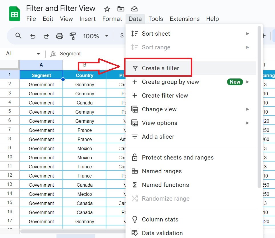
- Go to Data > Create a filter.
- A small filter icon appears in every header cell. Click one to open its filter menu.
To remove it later, use Data > Remove filter. All hidden rows come back.
Filter by Values (Text Columns)
Use this when you want to keep a few specific items, such as one segment.
- Click the filter icon in the Segment header.
- Under Filter by values, click Clear to untick everything.
- Tick only the values you want, for example Channel Partners, and click OK.
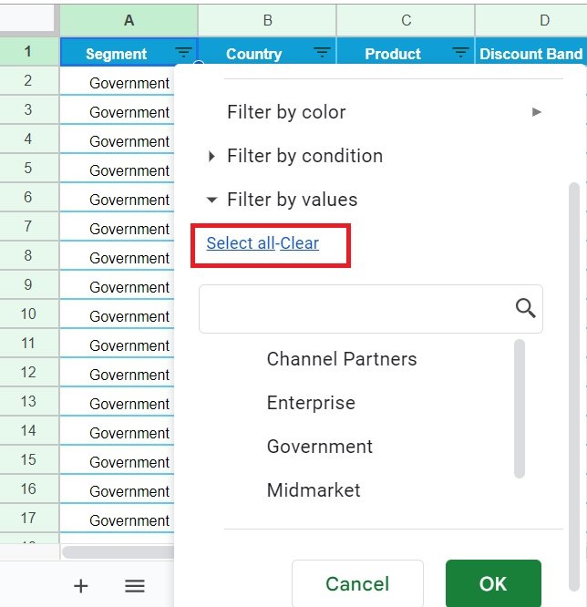
The search box above the list is handy when a column has dozens of values. Type part of a name and tick the matches.
Filter by Condition (Number Columns)
For numbers, conditions are faster than ticking values. To show only large orders:
- Open the filter menu on Units Sold.
- Expand Filter by condition and choose Greater than.
- Type
300and click OK.
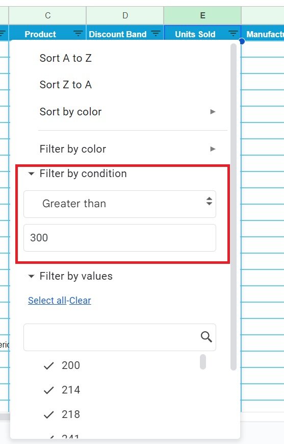
Other useful conditions include Less than, Is between, Is equal to, Is empty and Text contains. Date columns have their own options such as Date is before and Date is after, which is how you would narrow the Date column to one quarter.
Filter by Colour
If some cells are highlighted, you can show only those rows. In the practice file, a few COGS cells are filled light yellow.
- Open the filter menu on COGS.
- Go to Filter by color > Fill Color.
- Pick light yellow 3.
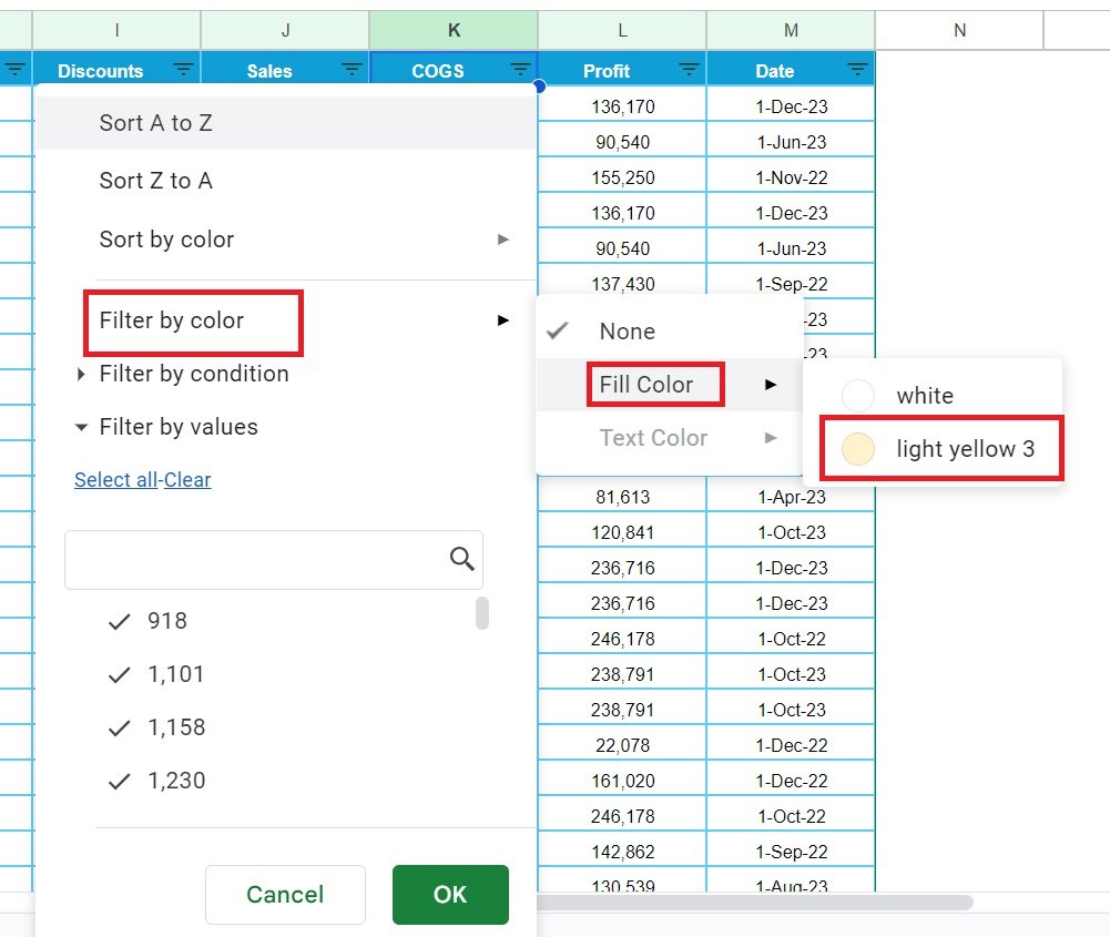
Colour filtering pairs well with conditional formatting: highlight exceptions with a rule, then filter on that colour to review them.
Filter With a Custom Formula
When one condition is not enough, use Filter by condition > Custom formula is. The formula is written for the first data row, and Sheets applies it to every row.
Worked example: show only Canada rows that sold more than 300 units. Open the filter on any column, choose Custom formula is and enter:
=AND($B2="Canada",$E2>300)Column B is Country and column E is Units Sold, so a row stays visible only when both tests return TRUE. A few more patterns you can paste in:
- Either of two countries:
=OR($B2="Canada",$B2="Mexico") - Profit above the column average:
=$L2>AVERAGE($L$2:$L) - Dates in 2023 only:
=YEAR($M2)=2023 - Product name starts with “V”:
=LEFT($C2,1)="V"
Filter Views: Filter Without Disturbing Others
On a shared sheet, a normal filter hides rows for everybody, which can be confusing. A filter view solves this.
- Go to Data > Create filter view. The row and column headers turn dark to show you are inside a filter view.
- Click the name box at the top left and give the view a clear name, for example Canada country.
- Apply filters and sorting as usual. Only you see the result.
- Close the view with the X at the top right. It is saved automatically.
If you already have a normal filter applied, Data > Save as filter view turns it into a filter view in one step.
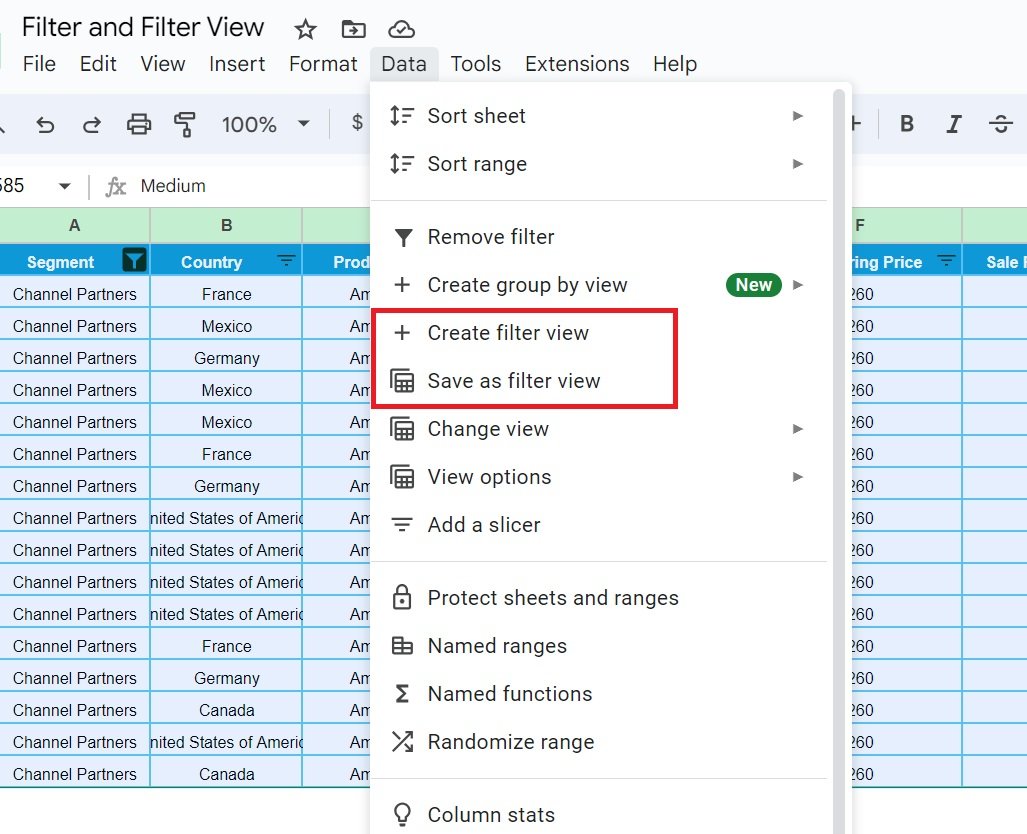
To reopen a saved view later, go to Data > Change view and pick it from the list. Each filter view also has its own URL, so you can send a colleague a link that opens the sheet already filtered.
Common Problems and Fixes
- New rows are not filtered. The filter range stopped at the old last row. Remove and recreate the filter, or select whole columns before creating it.
- A colleague says rows disappeared. Someone used a normal filter on a shared sheet. Clear it and use a filter view instead.
- The custom formula hides everything. Check that the formula refers to row 2 (the first data row) with the column locked, such as
$B2, notB$2. - Numbers will not filter by condition. They may be stored as text. Convert the column with Format > Number and try again.
- View-only users cannot create a normal filter. They can still create a temporary filter view that only they see.
Best Practices
- Keep one header row with no blank columns inside your data, so the filter covers everything.
- Name filter views by purpose (“Q4 Germany”, “Low profit check”) instead of leaving the default names.
- Combine filters on several columns (for example Segment plus Units Sold) for sharper questions.
- Use the FILTER function when the filtered list must feed another report automatically.
Want to go further? Learn the formula version in SORT and FILTER functions in Google Sheets and FILTER and ISBLANK in Google Sheets. To summarise the same data instead of just hiding rows, read the pivot table guide for Google Sheets, and see how filter and group-by views work inside tables in Google Sheets.
If you are new to spreadsheets and want a guided route through filters, formulas and reporting, the learning paths on NextGenTemplates Academy are a good place to start.
Frequently Asked Questions
What is the difference between a filter and a filter view in Google Sheets?
A filter changes the sheet for everyone who opens it. A filter view is a saved, personal filter that only affects your screen, so collaborators keep seeing the full data.
Are filter views saved automatically?
Yes. Once created, a filter view stays in the file. Reopen it any time from Data > Change view.
Can I share a filter view with someone?
Yes. While the view is open, copy the URL from the address bar. Anyone with access to the sheet who opens that link sees the same filtered view.
Can I apply more than one condition to a single column?
The built-in condition list allows one condition per column, but a custom formula such as =AND($E2>300,$E2<1000) lets you combine as many as you like.
Can view-only users filter a sheet?
They cannot change a normal filter, but they can create a temporary filter view for themselves. It disappears when they close it.
Does filtering delete any data?
No. Filters only hide rows. Remove the filter or close the filter view and every row is visible again.
Wrapping Up
Use a normal filter when you are working alone or want everyone to see the same subset, and a filter view whenever a sheet is shared. Between filtering by values, condition, colour and custom formula, you can answer most “show me only…” questions in a few clicks. Open the practice file and try each method on the sample sales data.
📅 Last updated: October 2026