Have you ever wondered how to quickly calculate the last day of the month based on any date? Whether you’re managing projects, bills, or just trying to keep track of important dates, the EOMONTH function in Google Sheets is a super handy tool. In this easy guide, I’ll show you how to use this function with a simple example. By the end, you’ll feel confident applying it in your own sheets. Let’s get started!
What is the EOMONTH Function?
First things first, let’s explain what the EOMONTH function does. This function helps you find the last day of the month either before or after a specific date, depending on the number of months you want to shift. It’s especially useful for things like calculating due dates or end-of-month deadlines.
=EOMONTH(start_date, months)
- start_ date: The date from which you want to start the calculation.
- months: The number of months you want to move forward or backward. Use positive numbers to move forward and negative numbers to move backward.
Now that we’ve covered the basics, let’s look at how you can apply this in real life!
Example Dataset
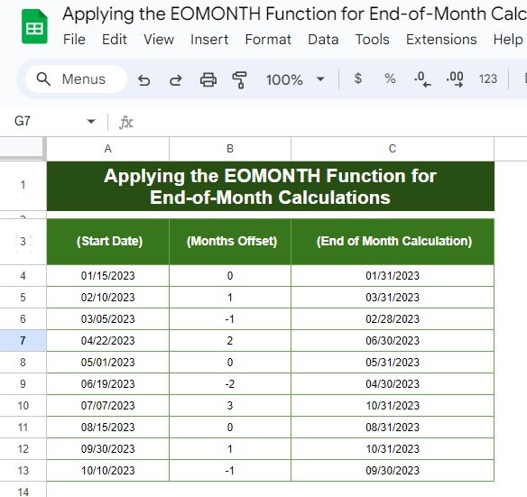
For our example, we have a dataset with start dates and a number of months to move. What we want to calculate is the end-of-month date for each of these start dates, considering how many months we’re shifting forward or backward.
The Goal:
We want to calculate the last day of the month for each start date using the EOMONTH function.
Step-by-Step Guide to Using the EOMONTH Function
Let’s walk through how to use the EOMONTH function step by step. Don’t worry—it’s super easy!
Pick the Cell for the Result
Start by selecting the first cell where you want the result to appear. For example, if your data is in column A, select C3.
Enter the Formula
Now, enter this formula into the selected cell:
=EOMONTH(A3, B3)
A3 is the start date you want to calculate from.
B3 is the number of months to shift (either forward or backward).
This formula will calculate the end of the month based on the start date and the months offset.
Copy the Formula for All Rows
Once you’ve entered the formula in the first row, you can easily apply it to the rest of the rows by dragging the small blue square in the corner of the cell down through the rest of the column. This will automatically calculate the end-of-month dates for all the rows in your dataset.
Understanding the Results
What Do These Results Mean?
When the Months Offset is 0, the function returns the last day of the same month as the start date. For example, 01/31/2023 for the date 01/15/2023.
When the offset is positive, the function moves forward by that many months. For instance, adding 1 month to 02/10/2023 gives you 03/31/2023.
A negative offset moves backward. For example, subtracting 1 month from 03/05/2023 results in 02/28/2023.
Why Should You Use the EOMONTH Function?
You might be wondering why this function is so helpful. Well, whether you’re managing deadlines, working on financial planning, or tracking project timelines, the EOMONTH function will save you tons of time. Here are a few reasons why you should start using it:
- Quickly Calculate End-of-Month Deadlines
This function allows you to effortlessly calculate the last day of any month, which is super useful when you need to meet deadlines, send out invoices, or set up reminders.
- Adjust Dates Forward or Backward
You can easily move dates forward or backward by adjusting the months offset, making it perfect for planning or reviewing past dates.
- Automate Repetitive Tasks
With just a simple formula, you can automate date calculations for large datasets, saving you from doing tedious manual work.
Final Thoughts
And there you have it—an easy and practical guide on how to use the EOMONTH function in Google Sheets! Whether you’re managing deadlines, invoices, or project timelines, this function will make your life so much easier. Give it a try in your own Google Sheets, and see how much time it saves you.
Visit our YouTube channel to learn step-by-step video tutorials
Youtube.com/@NeotechNavigators

