
Auto-Highlight Top 3 Students in Google Sheets Recognizing top-performing students is an essential task for educators and administrators. Google Sheets makes this task seamless by automating the process of highlighting the top 3 students in a dataset. In this article, you will learn how to use Google Sheets to Auto-Highlight the Top 3 Students with an example, step-by-step instructions, and creative tips to enhance your spreadsheet.
Why Auto-Highlight Top 3 Students in Google Sheets?
Highlighting the top performers not only makes data analysis more efficient but also provides a quick visual representation of achievements. This feature can be applied in:
Academic performance tracking
Corporate training results
Performance analysis in any field
Dataset for Example
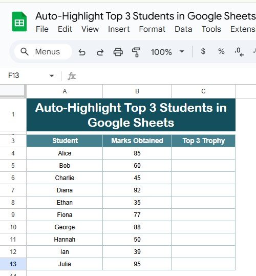
Let’s start with a sample dataset of students and their marks:
The goal is to identify the top 3 students based on their marks and add a trophy icon (🏆) in the “Top 3 Trophy” column.
Formula to Auto-Highlight Top 3 Students in Google Sheets
We’ll use the LARGE function in Google Sheets to identify the top 3 marks and the IF function to assign a trophy.
Formula:
=IF(B2>=LARGE($B$2:$B$11,3),"🏆","")
Explanation of the Formula:
- LARGE($B$2:$B$11,3): This function identifies the third highest value in the range $B$2:$B$11. It dynamically adjusts for the top three rankings.
- B2 >= LARGE($B$2:$B$11,3): Compares the marks in cell B2 with the third-highest value in the range.
- “🏆”: Assigns a trophy emoji if the condition is true.
- “”: Leaves the cell blank if the condition is false.
Step-by-Step Guide to Apply the Formula
Open Your Google Sheet
Load your dataset into Google Sheets.

Insert a New Column
Add a column labeled “Top 3 Trophy” to display the result.
Enter the Formula
In the first row of the “Top 3 Trophy” column, enter the formula:
=IF(B2>=LARGE($B$2:$B$11,3),”🏆”,””)
Drag the Formula Down
Copy the formula for all rows in the column by dragging it down.
Review the Output
The top 3 students will now have a trophy emoji displayed next to their names.
Output Example
After applying the formula, the dataset will look like this:


Advantages of Auto-Highlighting Top 3 Students
- Quick Recognition: Instantly identify the top performers without manual sorting.
- Improved Accuracy: Eliminate human error in ranking calculations.
- Dynamic Updates: The formula adjusts automatically as data changes.
- Visual Appeal: Highlighting with emojis or conditional formatting makes the data more engaging.
Opportunities for Improvement in Highlighting Top Performers
While this method is effective, there are areas where it can be enhanced:
- Custom Icons: Use other symbols or custom text for better representation (e.g., “Gold”, “Silver”, “Bronze”).
- Conditional Formatting: Pair the formula with conditional formatting to visually highlight the rows of the top 3 students.
- Dynamic Range Adjustments: Automate the range selection by using named ranges or dynamic arrays.
- Handling Ties: Adapt the formula to handle cases where multiple students have the same marks.
Best Practices for Auto-Highlighting in Google Sheets
- Keep Formulas Simple: Avoid overly complex formulas; break them down into helper columns if needed.
- Test with Sample Data: Validate the formula on a smaller dataset before applying it to larger ones.
- Use Conditional Formatting: Combine the formula with row-based conditional formatting to color-code the top performers.
- Document the Criteria: Clearly state the criteria for selection (e.g., top 3 based on marks) for transparency.
- Bonus: Using Conditional Formatting for Visual Impact
To further enhance the visualization of the top 3 students:
Highlight the “Marks Obtained” column.
Go to Format > Conditional Formatting.
Use the custom formula:
=B2>=LARGE($B$2:$B$11,3)
Choose a color (e.g., gold) to highlight the top 3 rows.
This approach adds an extra layer of visual emphasis.
Conclusion
Auto-highlighting the top 3 students in Google Sheets is a simple yet powerful technique for recognizing performance. By combining the LARGE function with IF, you can automate this task efficiently. Adding visual elements like emojis or conditional formatting makes your data stand out and provides immediate insights.
Frequently Asked Questions (FAQs)
- Can I use this formula for top 5 or top 10 students?
Yes! Modify the k value in the LARGE function to change the ranking. For example:
=IF(B2>=LARGE($B$2:$B$11,5),”🏆”,””)
- What happens if there’s a tie in marks?
The formula highlights all students with marks equal to or greater than the third-highest value, including ties.
- Can I use text instead of emojis?
Absolutely! Replace “🏆” with custom text like “Top Performer”:
=IF(B2>=LARGE($B$2:$B$11,3),”Top Performer”,””)
- How do I adjust the formula for larger datasets?
Extend the range ($B$2:$B$100 for 100 rows) to accommodate larger datasets.
- Can I highlight the entire row for top students?
Yes, use conditional formatting with the custom formula:
=$B2>=LARGE($B$2:$B$11,3)
Visit our YouTube channel to learn step-by-step video tutorials
Youtube.com/@NeotechNavigators