Have you ever needed to find the highest or largest values in a list and then pull related data in Google Sheets? If so, you’re in luck! In this blog post, we will explain how to use two powerful functions—Learn how to use XLOOKUP and LARGE functions in Google Sheets with a clear example to find top values and related data.—together in Google Sheets. By combining these functions, you can easily extract the largest values from a list and identify corresponding items.
Let’s get started and see how these functions work step-by-step!
Understanding the XLOOKUP and LARGE Functions
Before we dive into the example, let’s briefly explain what these two functions do:
- XLOOKUP: This function is used to search for a value in a range or array and return the corresponding value from another range. Think of it as an upgraded version of VLOOKUP.
- LARGE: This function returns the nth largest value from a range. So, if you need to find the largest, second largest, or third largest value in a list, the LARGE function has you covered.
Now that we have a basic understanding, let’s jump into a real example using some product data.
Example: Working with Product and Price Data
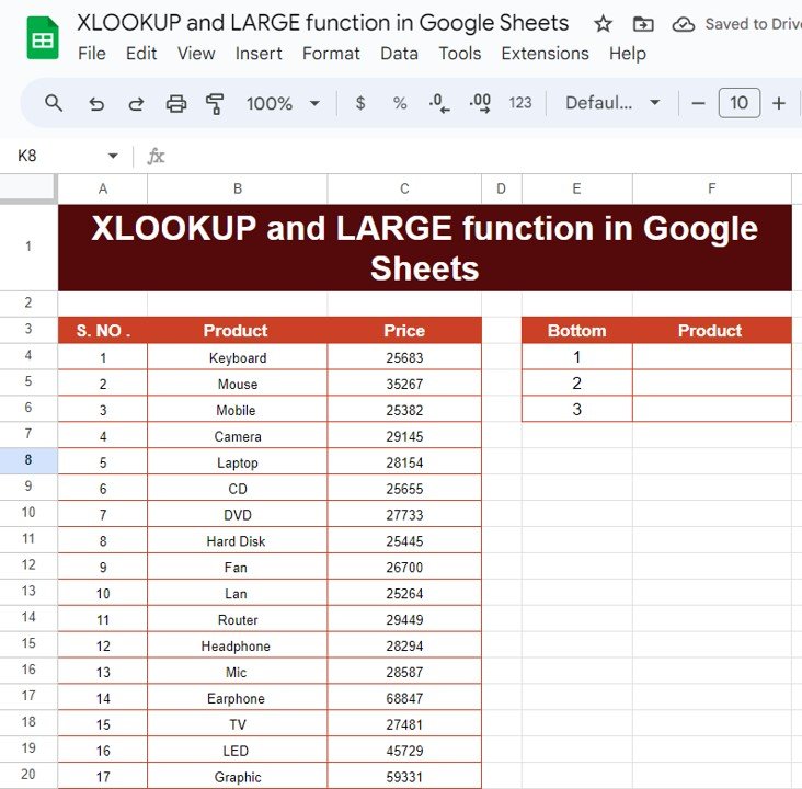
Here’s the dataset we’ll be using for this example. We have a list of products along with their prices. Our goal is to find the top-priced products using the XLOOKUP and LARGE functions.
Now, what we want to achieve is to pull the top-priced products and display them in order of their prices, from highest to lowest. For this, we’ll use the XLOOKUP and LARGE functions.

Step-by-Step Guide to Using XLOOKUP and LARGE Functions
- Using the LARGE Function to Find the Largest Prices
First, we’ll use the LARGE function to identify the highest prices in our dataset. Let’s say we want to find the top three highest prices. Here’s the formula you would use to get the largest price in cell E4:
=LARGE($C$4:$C$20,1)
In this formula, $C$4:$C$20 is the range that contains the product prices.
The 1 in the formula refers to the largest (or highest) value. If you wanted the second largest price, you would replace 1 with 2 and so on.
Apply the same formula for the next two highest prices by changing the 1 to 2 and 3 for the second and third largest prices respectively.
-
Using XLOOKUP to
Find the Product Names
Now that we have the top prices, it’s time to find the corresponding products using XLOOKUP. Here’s the formula for finding the product with the largest price:
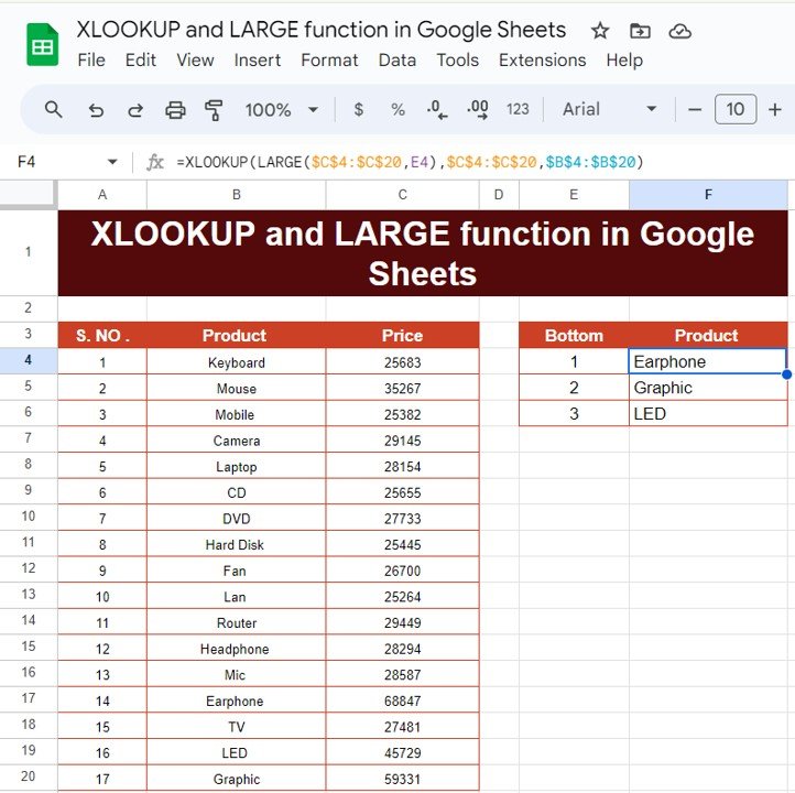
=XLOOKUP(LARGE($C$4:$C$20,E4),$C$4:$C$20,$B$4:$B$20)
Let’s break this down:
LARGE($C$4:$C$20,E4) finds the largest price in the range of prices, which we got in step one.
- $C$4:$C$20 is the range where we’re looking for the prices.
- $B$4:$B$20 is the range where the corresponding product names are located.
XLOOKUP then matches the largest price to the appropriate product.
-
Filling in the Remaining Products
Once you’ve applied this formula, drag it down to fill in the other cells for the second and third largest products. Now, you’ll have the top three highest-priced products along with their corresponding prices. Easy, right?
The Final Output
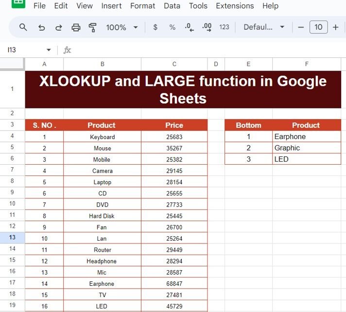
After applying both the XLOOKUP and LARGE functions, your output will look something like this:
These are the top three products with the highest prices from our list!

Why Use the XLOOKUP and LARGE Functions?
Now that you’ve seen how these two functions work together, you might be wondering why you should use them. Here are a few reasons why they’re so useful:
- Saves Time: You don’t have to manually search for the highest values or match them with their corresponding products. The formulas do the heavy lifting for you.
- Accurate Results: Using these functions ensures that you get accurate results without any manual errors.
- Efficient Data Management: If you’re working with large datasets, this combination of functions can make sorting and identifying key data points much easier.
Conclusion
And there you have it! By combining the XLOOKUP and LARGE functions in Google Sheets, you can easily find the top-priced items in any dataset. These two formulas are powerful tools that save you time and effort, especially when working with large amounts of data.
Visit our YouTube channel to learn step-by-step video tutorials
Youtube.com/@NeotechNavigators
Watch the step-by-step video tutorial:
Click here to Make the copy of this Template


