
Google Sheets is not just a tool; it’s a powerhouse for anyone eager to slice through data with precision. Among its myriad of features, VLOOKUP is a true standout, renowned for its knack to pinpoint exact data within mammoth datasets. Ready to revolutionize how you handle data? These six VLOOKUP hacks will not only boost your skills but also open up new avenues for using this versatile function.
Understanding Google Sheets Magic: 6 VLOOKUP Hacks That’ll Blow Your Mind!
What exactly is VLOOKUP? Known as Vertical Lookup, this function is the Swiss Army knife in Google Sheets that searches for a value in the first column of a range, then fetches a corresponding value from the same row in a specified column. It’s a game-changer for anyone juggling large tables, making data retrieval a breeze.
Mastering the Basics of Google Sheets Magic: 6 VLOOKUP Hacks That’ll Blow Your Mind!
Before we leap into more sophisticated tricks, let’s nail down the basics. Imagine you have a dataset with employee details such as ID, name, login hours, and calls handled. Here’s how you can perform a simple VLOOKUP:
The Perks of Becoming a VLOOKUP Pro
- Swift Data Retrieval: Instantly locate the exact piece of data you need within a sprawling dataset.
- Minimize Errors: Cut down on the mistakes that come with manual data searches.
- Elevate Data Manipulation: Seamlessly integrate VLOOKUP with other functions to handle complex data tasks without heavy scripting.
Where VLOOKUP Could Do Better
Despite its power, VLOOKUP isn’t without its limitations—it only searches rightward across columns. But, don’t worry! Recognizing these limits can help you leverage its strengths even better.
VLOOKUP Best Practices
- Accuracy is Key: Always double-check your search key is unique to sidestep fetching incorrect data.
- Smart Data Layout: Keep your searchable data in the leftmost columns to maximize VLOOKUP’s efficiency.
- Lock It Down: Use absolute references (like $A$2:$E$11) in your range to avoid errors when copying formulas.
6 Mind-Blowing VLOOKUP Hacks
- Normal VLOOKUP
The standard VLOOKUP function searches for a value in the first column of a specified range and returns a value in the same row from a different column you specify.

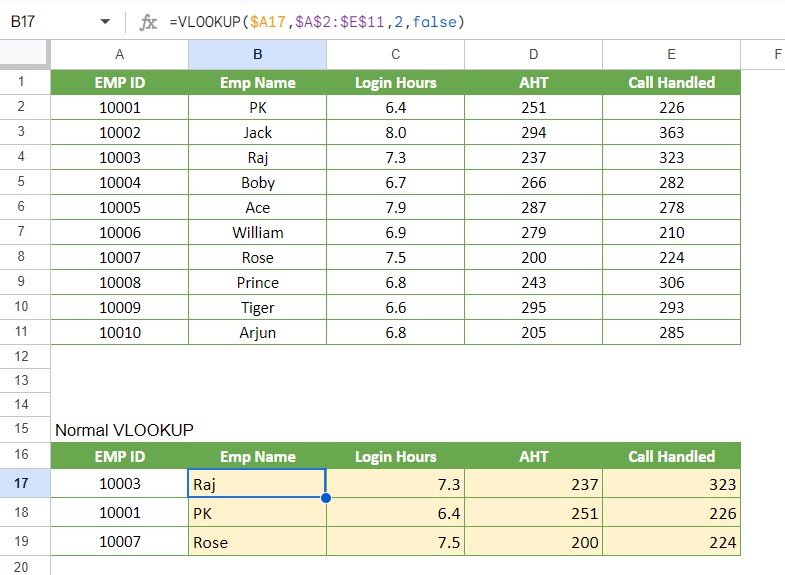
Syntax Example:
=VLOOKUP(10003, A2:E10, 3, FALSE)
This searches for the ID 10003 and returns the value from the third column of the range A2:E10.
- VLOOKUP with COLUMN()
This variation uses the COLUMN function to dynamically specify which column to return data from, making your VLOOKUP adaptable to changes in the spreadsheet’s structure.

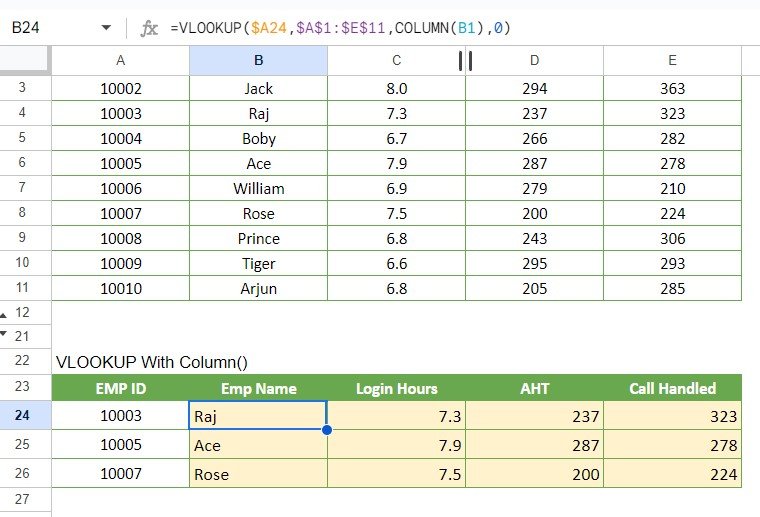
Syntax Example:
=VLOOKUP(10003, A2:E10, COLUMN(D1), FALSE)
This finds 10003 in the range and returns the value from the column where D1 is located, dynamically adjusting if columns are added or removed.
- VLOOKUP with MATCH
Combining VLOOKUP with MATCH allows you to dynamically locate both the lookup value and the column index, providing flexibility when column positions might change.
Syntax Example:
=VLOOKUP(10003, A2:E10, MATCH("Login Hours", A1:E1, 0), FALSE)
This searches for 10003 and returns the value from the column labeled “Login Hours,” regardless of its position in the row.
- Double VLOOKUP
A double VLOOKUP is useful when you need to perform a sequential lookup, such as when the result of the first VLOOKUP serves as the lookup value for the second VLOOKUP.

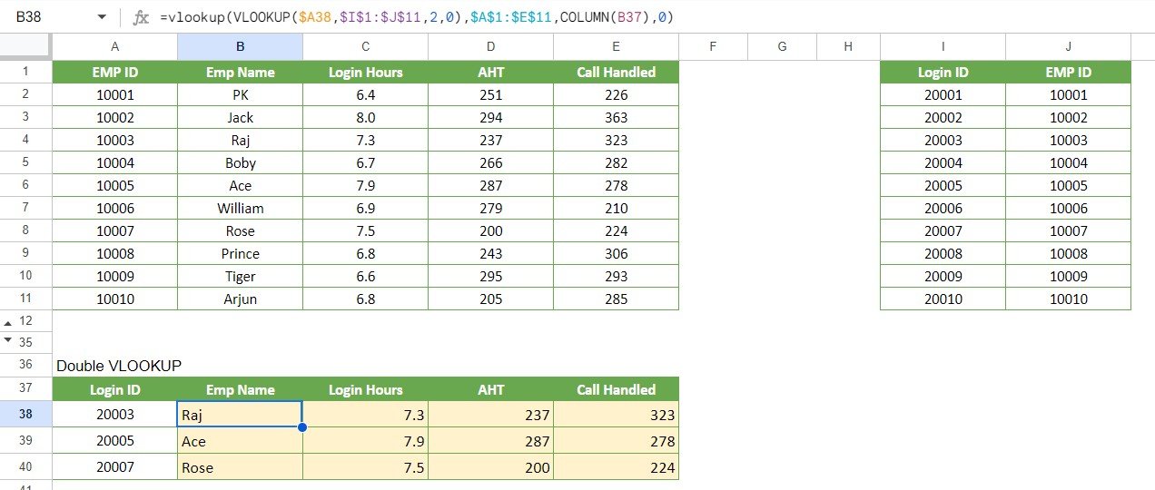
Syntax Example:
=VLOOKUP(VLOOKUP(20003, A2:B10, 2, FALSE), C2:D10, 2, FALSE)
This first finds 20003 and uses the result to perform another VLOOKUP in a different range.
- Error Handling in VLOOKUP
Using IFERROR with VLOOKUP ensures that you handle errors gracefully, providing a default value when VLOOKUP fails to find the lookup value.

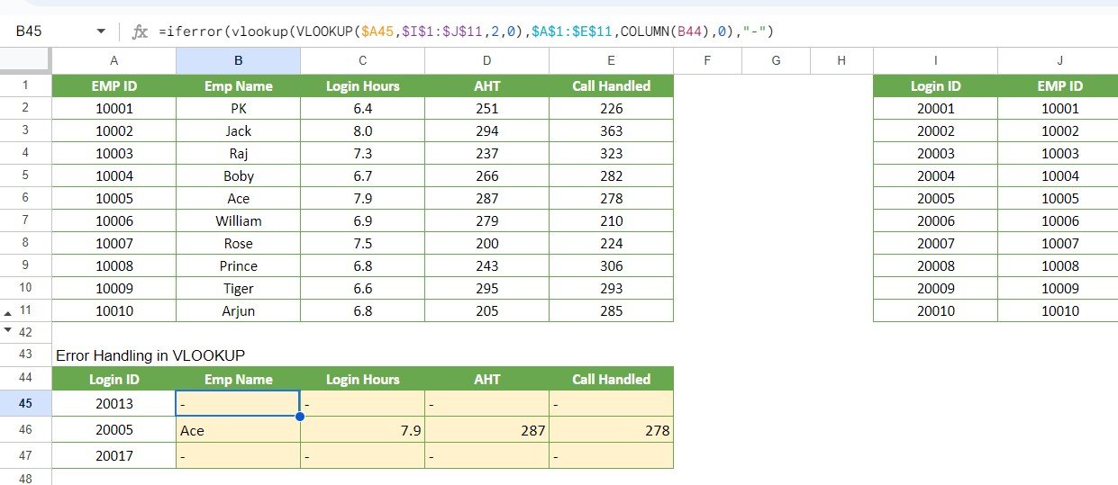
Syntax Example:
=IFERROR(VLOOKUP(20013, A2:E10, 2, FALSE), "Not Found")
This returns “Not Found” instead of an error if 20013 isn’t located, improving the user experience.
- Ageing/Buckets with VLOOKUP
This hack is used to categorize or classify data based on age or other criteria, returning the category into which the data falls. It’s particularly useful for financial analysis or inventory management.

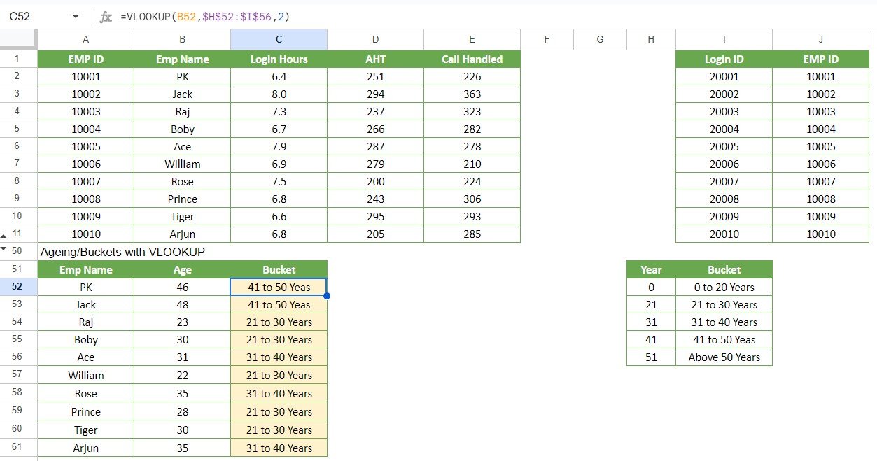
Syntax Example:
=VLOOKUP(E2, Age_Range_Table, 2, TRUE)
Here, E2 contains an age, and Averageable has predefined age buckets. VLOOKUP returns the age bucket in which the age falls.
Your VLOOKUP Questions Answered
Q: Can VLOOKUP search from right to left?
A: No, it can’t. To search from right to left, consider using INDEX/MATCH instead.
Q: How can I make VLOOKUP return values from multiple columns?
A: Directly, you can’t with VLOOKUP. You’d need to use multiple VLOOKUPs or switch to INDEX/MATCH for that flexibility.
Q: What happens if VLOOKUP doesn’t find the lookup value?
A: It returns #N/A. To manage this, wrap your VLOOKUP in an IFERROR function to display a custom message instead of an error.
Embrace these techniques, and you’ll find yourself navigating through Google Sheets like never before. Enjoy your journey into the world of efficient data manipulation with VLOOKUP!
Visit our YouTube channel to learn step-by-step video tutorials
Youtube.com/@NeotechNavigators
Watch the step-by-step video tutorial:
