Have you ever wanted to create a rating system in Google Sheets using stars? Whether it’s for product reviews, employee feedback, or any type of rating system, this guide will show you how to easily create a star rating using the REPT function in Google Sheets.
In this post, we’ll walk you through the process using a real-life example. By the end, you’ll have the skills to generate a dynamic star rating system that can be customized for your own needs. Let’s dive in!
What is the REPT Function in Google Sheets?
Before we get into the example, let’s talk about the REPT function. This handy function allows you to repeat a specific character or string a set number of times. It’s incredibly useful when you need to create patterns or visual elements like stars for a rating system.
The syntax is simple:
=REPT(text, number _of_ times)
For our star rating, we’ll use the REPT function to repeat the star symbol (⭐) based on the rating score provided in the data. Now, let’s see how to apply it!
Data for Our Example
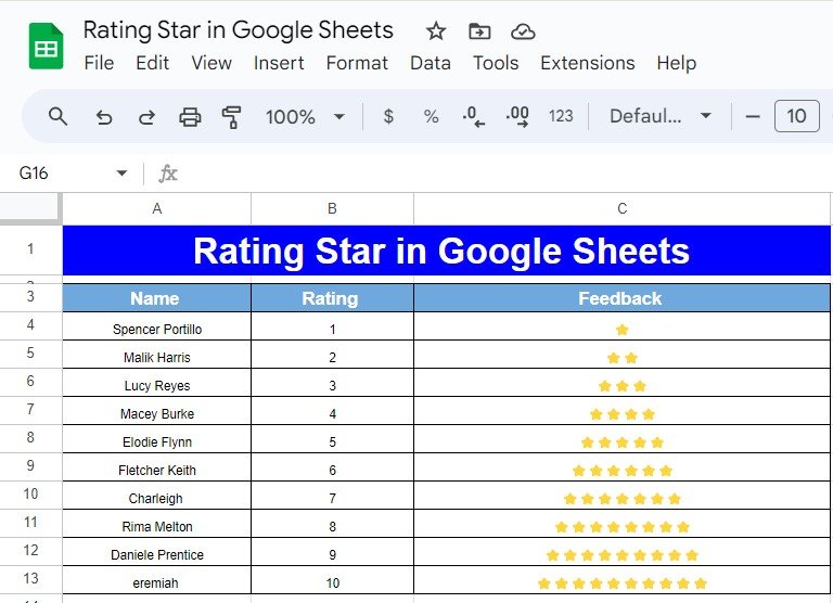
We have a small dataset consisting of names and their corresponding ratings. Here’s a sample of what the data looks like:
As you can see, each person has a rating from 1 to 10, and we want to display their feedback using stars.
How to Create a Star Rating with the REPT Function
Now, let’s get to the fun part—using the REPT function to create the star rating. Here’s the formula we’ll use:
=REPT("⭐", B4)

Explanation of the Formula:
REPT(“⭐”, B4): The REPT function repeats the star symbol (⭐) as many times as the number in cell B4 (which contains the rating).
For example:
If B4 contains 1, the formula returns ⭐.
If B4 contains 2, the formula returns ⭐⭐.
And so on, until you reach 10 stars for a rating of 10.
With this formula, you’ll be able to visually represent each person’s rating with stars in the “Feedback” column.
Step-by-Step Process
Set up your data:
You should have a dataset similar to the one above, with a “Name” column, a “Rating” column, and an empty “Feedback” column where we’ll display the star ratings.
Insert the REPT formula:
In the first cell of the “Feedback” column (e.g., C3), type the following formula:
=REPT("⭐", B3)
This formula will display one star for a rating of 1, two stars for a rating of 2, and so on.
Drag the formula down:
After entering the formula, click on the small blue box at the bottom-right corner of the cell and drag it down to fill the rest of the column. Now, you’ll see the star ratings for all entries.
What Does the Output Look Like?
Once you’ve applied the formula, your Google Sheet will look something like this:
This simple formula creates a visually appealing rating system that’s both functional and easy to understand.

Final Thoughts
Creating a star rating in Google Sheets is quick and easy with the REPT function. This method can be applied to many other use cases, such as performance evaluations, product ratings, or customer satisfaction scores. Try experimenting with different symbols or applying conditional formatting to enhance the look even further!
Visit our YouTube channel to learn step-by-step video tutorials
Youtube.com/@NeotechNavigators
View this post on Instagram


