


Google Sheets has become one of the most widely used tools for organizing data, performing calculations, and collaborating with others. Whether you’re a beginner looking to get started or an advanced user aiming to refine your skills, these life-changing tips will help you master Google Sheets in no time.
In this article, we will cover essential tips and tricks that will enhance your productivity and help you unlock the full potential of Google Sheets. Let’s dive into the strategies that will transform the way you work with spreadsheets.
Why Google Sheets is the Ultimate Spreadsheet Tool
Before we get into the tips, let’s take a moment to appreciate why Google Sheets is such a powerful tool for individuals and businesses alike.
- Cloud-Based: Since Google Sheets is cloud-based, you can access your work from anywhere at any time. There is no need to worry about losing your data due to hardware failure or forgetting to save your work.
- Collaborative Features: You can collaborate with others in real-time, making it an excellent tool for team projects and business-related tasks.
- User-Friendly: Google Sheets offers a user-friendly interface that doesn’t require an advanced level of expertise, making it easy to get started and get things done quickly.
- Integrations and Add-ons: Google Sheets allows seamless integration with other Google apps and third-party add-ons, enabling you to automate tasks, analyze data, and extend its functionality.
Now, let’s explore life-changing tips that will help you master Google Sheets and boost your productivity.
Use Keyboard Shortcuts for Faster Navigation
Google Sheets, like many other Google apps, comes with a variety of keyboard shortcuts that can significantly speed up your workflow. By using shortcuts, you can navigate through your spreadsheet, perform actions, and edit data without ever needing to leave the keyboard. Here are some essential shortcuts to remember:
Key Shortcuts to Speed Up Your Work:
- Ctrl + Z: Undo the previous action.
- Ctrl + Shift + Z: Redo the last action.
- Ctrl + C: Copy the selected cell or range of cells.
- Ctrl + V: Paste the copied cells.
- Ctrl + X: Cut the selected cells.
- Ctrl + Shift + V: Paste only the values, not the formatting.
- Ctrl + Arrow Key: Move to the edge of the data range.
- Ctrl + Space: Select the entire column.
- Shift + Space: Select the entire row.
By mastering these shortcuts, you can complete tasks more efficiently and save valuable time while working in Google Sheets.
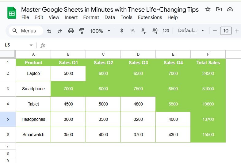
Leverage Conditional Formatting for Better Data Visualization
One of the most powerful features of Google Sheets is conditional formatting. This feature allows you to automatically apply different formats (such as colors, fonts, or borders) based on the data in your cells. By using conditional formatting, you can make your data visually appealing and easier to interpret.
How to Apply Conditional Formatting:
- Highlight Data: Select the range of cells you want to format.
- Go to Format > Conditional Formatting: This will open a panel on the right.
- Choose a Format Rule: You can select options like “Greater than,” “Text contains,” or “Custom formula” to set the conditions.

- Pick a Formatting Style: Choose the color or style you want to apply when the condition is met.
This feature can be particularly useful when you want to highlight trends, identify outliers, or draw attention to important information. For example, you can use conditional formatting to change the background color of a cell when a sales figure exceeds a specific target.
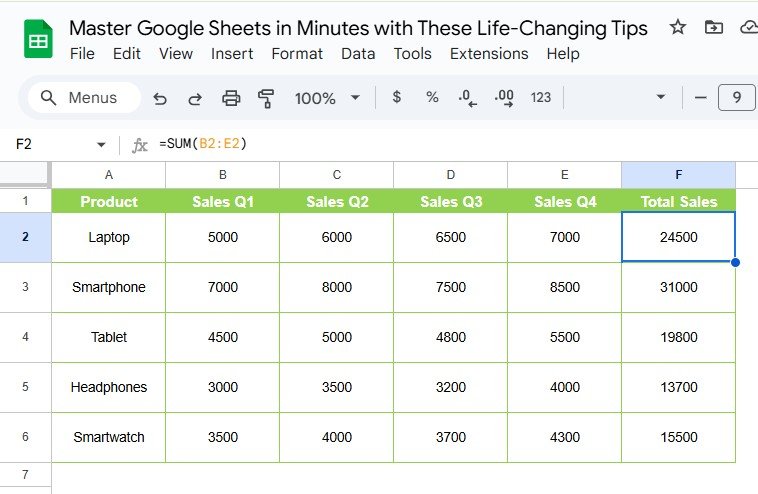
Master Functions to Automate Calculations
Functions are the backbone of Google Sheets, enabling you to perform complex calculations with minimal effort. The more functions you know, the easier it will be to manage and analyze data. Here are some essential functions you should get familiar with:
Commonly Used Functions in Google Sheets:
- SUM: Adds up all the values in a range of cells.
=SUM(A1:A10)

- AVERAGE: Calculates the average of a range of cells.
=AVERAGE(A1:A10) - VLOOKUP: Searches for a value in the first column of a range and returns a value from another column in the same row.
=VLOOKUP(A2, B1:C10, 2, FALSE) - IF: Checks whether a condition is met and returns one value if true and another if false.
=IF(A1 > 10, “Yes”, “No”) - COUNTIF: Counts the number of cells that meet a specific condition.
=COUNTIF(A1:A10, “>10”) - INDEX/MATCH: A powerful combination of functions used to perform lookups more flexibly than VLOOKUP.
=INDEX(A1:A10, MATCH(“value”, B1:B10, 0))
These functions can help you automate repetitive tasks, saving you hours of manual calculations and ensuring the accuracy of your work.
Collaborate with Others in Real-Time
One of the standout features of Google Sheets is its real-time collaboration. Whether you’re working on a team project or sharing data with a client, you can collaborate on the same document simultaneously.
How to Collaborate Effectively in Google Sheets:
- Share Your Spreadsheet: Click on the Share button in the top right corner, and add email addresses to give others access to the sheet.
- Set Permissions: Choose whether the collaborators can view, comment, or edit the spreadsheet.
- Use Comments and Notes: Highlight a cell, right-click, and choose Comment to leave feedback or suggestions for others. You can also use Notes to add context to a cell without sharing it with everyone.
- Version History: If you’re working with multiple people, use File > Version History > See Version History to view past changes and revert to previous versions of the document if necessary.
By leveraging these collaboration features, you can seamlessly work together with your team, receive feedback, and track changes without confusion.
Create Dynamic Dashboards for Data Analysis
Google Sheets allows you to create powerful dashboards that allow you to analyze data visually. You can combine charts, pivot tables, and other features to create an interactive and insightful data dashboard.
Steps to Create a Dynamic Dashboard:
- Organize Your Data: Ensure your data is well-organized in columns and rows with clear headers.
- Use Pivot Tables: Pivot tables allow you to quickly summarize large sets of data and create dynamic reports. To create a pivot table, go to Data > Pivot Table.
- Insert Charts: Visualize your data by selecting your desired range and clicking Insert > Chart. Choose from various chart types such as bar charts, pie charts, and line charts.
- Filter Data: Use Data > Filter Views to create different views of the data without affecting others.
- Use Slicers: Add slicers to your dashboard to make it interactive. Slicers allow users to filter data by different categories, making it easier to analyze trends.
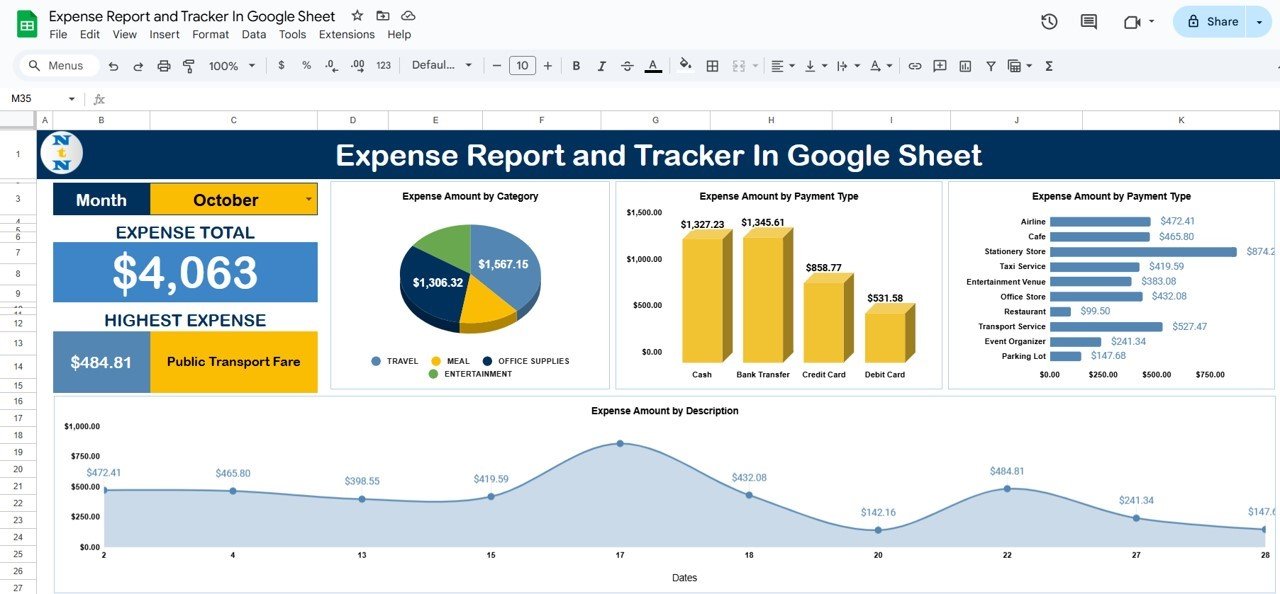

A dynamic dashboard makes it simple to present data in a clear and engaging way, providing valuable insights at a glance.
Conclusion
Google Sheets is a versatile and powerful tool that can help you organize data, automate tasks, and collaborate with others. By incorporating these life-changing tips into your workflow, you’ll become more efficient and productive in no time. From using keyboard shortcuts and mastering functions to collaborating in real-time and creating dynamic dashboards, these tips will help you unlock the full potential of Google Sheets.
Visit our YouTube channel to learn step-by-step video tutorials
Youtube.com/@NeotechNavigators