

Google Sheets is a powerhouse for data management, and knowing how to combine formulas can boost productivity and automate tasks effortlessly. Here are five secret formula combinations that will transform the way you use Secret Formula Combos to Supercharge Your Google Sheets
INDEX + MATCH for More Flexible Lookups
Forget VLOOKUP – this combo is more powerful!
Why Use It?
Works with columns in any position (unlike VLOOKUP).
More accurate and dynamic.
Example: Find an Employee’s Salary Based on Their ID
=INDEX(B2:B100, MATCH(E2, A2:A100, 0))
How It Works:
- MATCH(E2, A2:A100, 0) finds the row number where E2 (employee ID) exists.
- INDEX(B2:B100, row_number) returns the salary from column B.

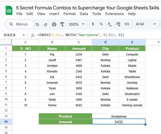
Supercharge Your Skills: Use this when the lookup column isn’t the first column in your dataset.
ARRAYFORMULA + IF for Bulk Conditional Operations
Save time by applying formulas across an entire column without dragging!
Why Use It?
Automates calculations for large datasets.
Works great with IF conditions.
Example: Calculate Bonuses for Employees Earning Above $5000
=ARRAYFORMULA(IF(B2:B100 > 5000, B2:B100 * 0.1, 0))
How It Works:
- Checks if each value in B2:B100 is greater than 5000.
- If true, applies 10% bonus; otherwise, returns 0.
Supercharge Your Skills: Use ARRAYFORMULA with TEXT, LEN, and SUBSTITUTE for bulk text transformations.
QUERY + IMPORTRANGE to Analyze Data from Another Sheet
Combine data from different spreadsheets without copy-pasting!
Why Use It?
Fetches data from an external Google Sheets file.
Performs sorting, filtering, and calculations dynamically.
Example: Import and Summarize Sales Data from Another Spreadsheet
=QUERY(IMPORTRANGE("SpreadsheetURL", "Sheet1!A1:C100"), "SELECT Col1, SUM(Col3) WHERE Col2 = 'Product A' GROUP BY Col1")
How It Works:
- IMPORTRANGE(“SpreadsheetURL”, “Sheet1!A1:C100”) fetches data from another Google Sheet.
- QUERY(…, “SELECT Col1, SUM(Col3) WHERE Col2 = ‘Product A’ GROUP BY Col1”) filters and summarizes sales data for “Product A”.
Supercharge Your Skills: Modify the QUERY statement to perform advanced analytics across multiple datasets!
TEXTJOIN + FILTER for Smart Data Consolidation
Need to combine multiple values based on a condition? This trick is gold!
Why Use It?
Merges multiple results into a single cell.
Works great for creating dynamic lists.
Example: List All Employees in the Sales Department
=TEXTJOIN(", ", TRUE, FILTER(A2:A100, B2:B100 = "Sales"))
How It Works:
- FILTER(A2:A100, B2:B100 = “Sales”) extracts all names from the “Sales” department.
- TEXTJOIN(“, “, TRUE, …) joins the results into one cell, separated by “, “.
Supercharge Your Skills: Modify the FILTER criteria to build custom reports dynamically!
GOOGLETRANSLATE + ARRAYFORMULA to Translate Entire Columns
Want to instantly translate multiple rows of text? Automate it!
Why Use It?
Translates bulk text in seconds.
Works with any Google-supported language.
Example: Translate Column A from English to Spanish
=ARRAYFORMULA(GOOGLETRANSLATE(A2:A100, "en", "es"))
How It Works:
- GOOGLETRANSLATE(A2:A100, “en”, “es”) translates each value in column A from English to Spanish.
- ARRAYFORMULA(…) applies the translation to all rows automatically.
Supercharge Your Skills: Change “es” to other language codes (e.g., “fr” for French, “de” for German).
Final Thoughts
These 5 formula combinations will save you time, automate tasks, and take your Google Sheets skills to the next level!
What’s Next?
- Try them in your own spreadsheets.
- Experiment with modifying conditions for your use case.
- Share this guide with your team to boost productivity!
Visit our YouTube channel to learn step-by-step video tutorials
Youtube.com/@NeotechNavigators