
If you’ve ever worked with trigonometric functions in Google Sheets, you may have come across the ACOS function. This powerful tool calculates the inverse cosine (arccosine) of a given number, returning the angle in radians. You can even convert the result to degrees with another simple formula. In this post, we’ll show you exactly how to use the ACOS function in Google Sheets, complete with an easy-to-follow example.
So, whether you’re handling data analysis, working on mathematical problems, or just exploring Google Sheets’ advanced functions, this blog post will guide you through the process in a simple, straightforward way.
What is the ACOS Function in Google Sheets?
The ACOS function in Google Sheets calculates the inverse of the cosine of a number, often referred to as arccosine. This function is particularly useful when you want to find the angle (in radians) that corresponds to a given cosine value. Here’s the basic syntax of the function:
=ACOS(value)
value: This is the number whose arccosine you want to calculate. It must be between -1 and 1 (inclusive), because cosine values can only fall within this range.
The result is returned in radians. However, if you want to convert this to degrees, you’ll need to apply an additional function, which we’ll explain in the next section.
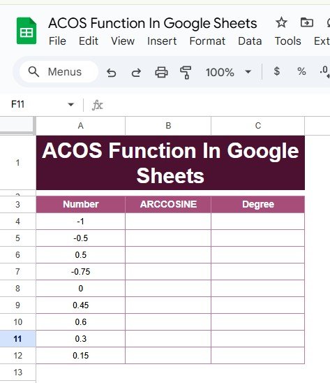
Example Data for Using the ACOS Function
Let’s dive into an example to see the ACOS function in action. Below is the data we’ll use for this demonstration:
How to Use the ACOS Function in Google Sheets
In this section, we’ll walk through how to use the ACOS function step by step. Here’s how you can calculate the inverse cosine for a number in your Google Sheets:
Step 1: Enter Your Data
First, you need to have a column with the numbers for which you want to calculate the arccosine (inverse cosine). In our example, the numbers are already listed in Column A.

Step 2: Apply the ACOS Formula
Next, to calculate the arccosine in radians, use the following formula:
=ACOS(A4)
For example, if you want to calculate the arccosine of the value in cell A4 (which contains -1), simply type the formula into the adjacent cell in Column B. This will give you the arccosine in radians.


Step 3: Convert Radians to Degrees
By default, the ACOS function returns the result in radians. If you want the result in degrees, you can use the DEGREES function to convert the radians value. The formula would look like this:
=DEGREES(B4)
In this case, assuming B4 contains the result from the ACOS formula, this will convert the radians to degrees.


Step 4: Review the Output
Once you’ve applied the formulas, your sheet will look something like this:


Explanation of the Formula
Let’s break down the formulas and understand what each part does:
- ACOS(A4): The ACOS function takes the value from cell A4 (in our case, -1) and calculates the inverse cosine of that value in radians.
- DEGREES(B4): The DEGREES function converts the radians value from cell B4 into degrees. This is useful when you want to interpret the result in a more familiar unit, as degrees are often easier to understand in many practical situations.
For instance, the arccosine of -1 is π radians, which equals 180 degrees. That’s exactly what our output shows.
Practical Applications of the ACOS Function
Now that we know how to use the ACOS function in Google Sheets, let’s talk about some practical applications:
- Data Analysis: If you’re working with angles or trigonometric data (like in physics or engineering), the ACOS function can help you quickly find angles from cosine values.
- Graphics and Design: For anyone working with 3D graphics or game development, understanding angles between vectors often requires using inverse trigonometric functions like ACOS.
- Statistical Models: ACOS can also be used when working with models that require calculating angles between data points or variables.
Conclusion
The ACOS function in Google Sheets is an incredibly useful tool when you need to calculate the arccosine (inverse cosine) of a number. By understanding the steps outlined above, you can easily compute the inverse cosine in both radians and degrees.
Visit our YouTube channel to learn step-by-step video tutorials
Youtube.com/@NeotechNavigators