Have you ever needed to figure out if a cell in Google Sheets contains a number or not? Well, there’s a super easy way to do this using the ISNUMBER function! In this blog post, I’ll walk you through how to update a table using this handy function, and by the end, you’ll know exactly how to tell whether a cell holds a number or something else, like text. Let’s jump right in!
What is the ISNUMBER Function?
Before we dive into the steps, let’s first talk about what the ISNUMBER function actually does. This function is designed to check if a value in a cell is a number. If the cell contains a number, it will return TRUE, and if it contains text or any non-numeric value, it will return FALSE. It’s super useful when you need to quickly sort through your data to find which values are numbers.
The Basic Syntax:
=ISNUMBER(value)
- value: This can be a specific cell or value you want to check.
Now that you have a clear idea of what this function is all about, let’s move on to a real-world example. Don’t worry, it’s easier than you think!
Example Dataset
For this example, let’s say we have some sample data ranging from A3
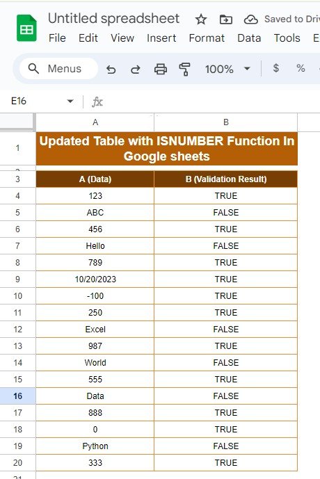
in our Google Sheet. In the A column, we have a mix of numbers, text, and dates. What we want to do is use the ISNUMBER function in the B column to check whether each value in column A is a number or not.
Here’s What Our Data Looks Like:
Now, let’s move on to how to apply the ISNUMBER function to this data.
How to Use the ISNUMBER Function in Google Sheets
Alright, here’s the fun part! Follow these simple steps, and you’ll have the validation done in no time.
Pick the Cell Where You Want the Result
First, go to the B4 cell, which is the first cell in the B column where we’ll apply the formula.
Type in the Formula
In B4, type the following formula:
=ISNUMBER(A4)
What this does is check whether the value in A4 (which could be a number, text, or date) is a number.
Fill the Rest of the Column
Once you’ve typed the formula, you don’t need to repeat it for every cell. Just drag the small blue square from the corner of B4 down to the rest of the cells in column B (B5
). This will apply the formula to all the rows automatically.
What Does the Result Look Like?
After you’ve applied the formula, this is what your table should look like:
What Does This Mean?
When the ISNUMBER function returns TRUE, it means the cell contains a number, like 123, 456, or even a date like 10/20/2023.
When it returns FALSE, it means the value is text, like ABC, Hello, or Excel.
Why Should You Use the ISNUMBER Function?
Now that you’ve seen how easy it is to use the ISNUMBER function, let’s talk about why it’s so useful! Whether you’re working with large datasets or just trying to keep your data organized, this function helps you quickly identify which values are numbers and which ones aren’t.
Here are a few reasons to start using it:
- Validate Data Quickly: The ISNUMBER function makes it simple to check if a cell contains a number, helping you avoid errors in your formulas or calculations.
- Find Non-Numeric Values Fast: M It’s much quicker than manually scanning through your data to see what’s a number and what’s text.
- Save Time with Automation: Once you’ve entered the formula, it takes care of the rest, checking every value for you. You’ll never have to do it manually again!
Final Thoughts
And there you have it—an easy-to-follow guide on how to use the ISNUMBER function in Google Sheets! Whether you’re sorting through customer data, validating numeric entries, or just cleaning up a messy spreadsheet, this function will make your life much easier. Now go ahead and give it a try in your next project!
Visit our YouTube channel to learn step-by-step video tutorials
Youtube.com/@NeotechNavigators

