Google Sheets is packed with a range of powerful functions that help simplify your workflow, and two of the most frequently used functions are VLOOKUP with COLUMN Function. Today, we are going to dive into how you can combine these two functions to enhance your data lookup capabilities in Google Sheets. By the end of this post, you’ll understand exactly how to use VLOOKUP with COLUMN in Google Sheets through a clear and practical example.
What is VLOOKUP in Google Sheets?
If you’ve ever worked with Google Sheets, you’ve likely come across the VLOOKUP function. In simple terms, VLOOKUP (Vertical Lookup) helps you search for a specific value in a column and return a corresponding value from another column in the same row. It’s an excellent tool for finding and organizing your data.
However, it can get even more powerful when combined with the COLUMN function. Let me explain how!
What is the COLUMN Function?
The COLUMN function in Google Sheets returns the column number of a specified cell or range of cells. For example, if you want to find out what column “C” belongs to, using =COLUMN(C1) will return “3” since “C” is the third column.
Now, when you use VLOOKUP with COLUMN, it can automatically adjust which column to fetch the data from, making your formulas dynamic and versatile.
Our Example Data
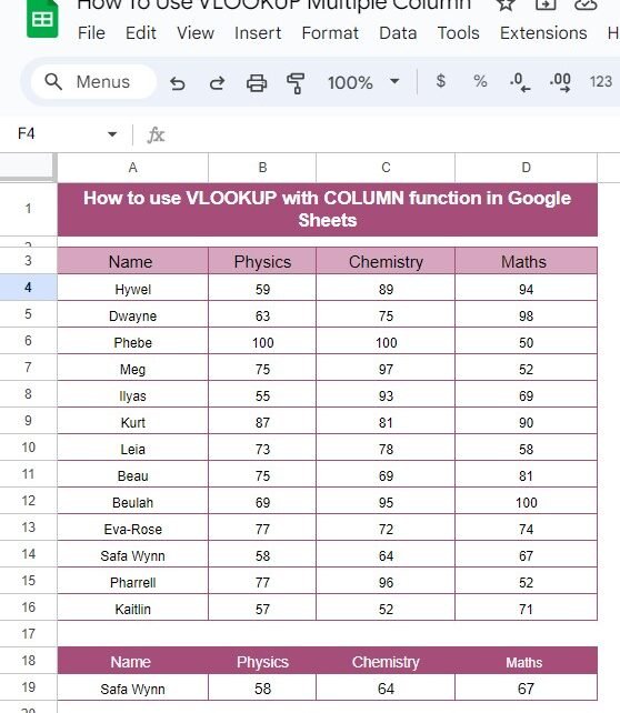
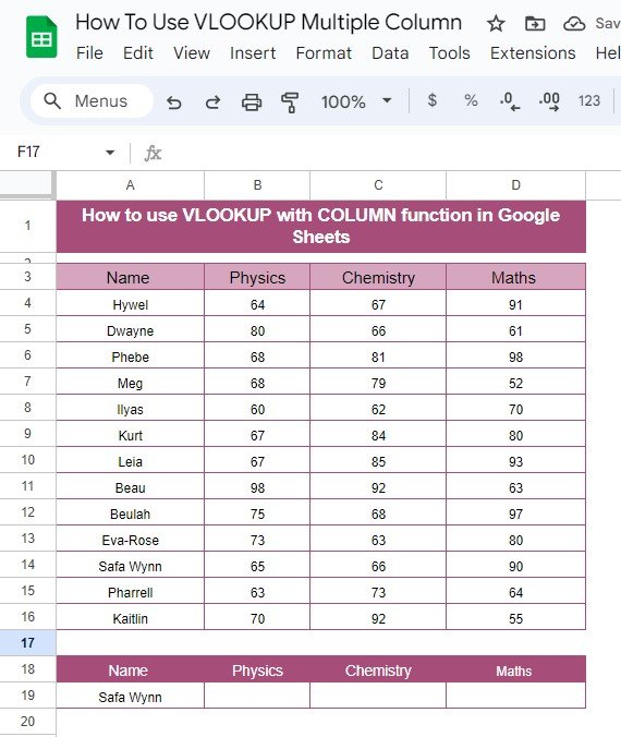
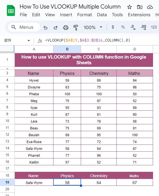
To understand how this combination works, we will use the following dataset of student scores in three subjects: Physics, Chemistry, and Maths.
We want to use VLOOKUP with COLUMN to dynamically find the data for any student we specify. Let’s say we’re particularly interested in looking up Safa Wynn’s marks from this table.
The Formula to Use
Here is the formula that will help you find the information you need:
=VLOOKUP($A$19,$A$3:$D$16,COLUMN(),0)
Breaking Down the Formula
VLOOKUP($A$19, $A$3:$D$16, COLUMN(), 0):
- $A$19: This is where we will input the name of the student whose scores we want to retrieve. In this case, let’s say Safa Wynn.
- $A$3:$D$16: This is the range where our data is stored. It covers the names and the three subjects.
- COLUMN(): This automatically adjusts to return the relevant column for Physics, Chemistry, or Maths based on where you place the formula.
- 0: This tells the VLOOKUP to perform an exact match, meaning it will look for an exact match for the name entered.
How Does the Formula Work?
When you input “Safa Wynn” in cell A19, the VLOOKUP function searches the first column (Name) in the range A3
for an exact match. It then returns the relevant data from either the Physics, Chemistry, or Maths column, depending on the current column the formula is in. Using the COLUMN() function makes this possible without needing to manually adjust the column index every time.
The Result
When you use this formula, the output will look like this:
The formula has dynamically pulled the data for Safa Wynn, and you can now see their scores in Physics, Chemistry, and Maths!
Why This Combination is Powerful
There are several reasons why combining VLOOKUP with COLUMN is a game-changer for working with data in Google Sheets:
- Automation: No need to manually change the column index when copying the formula across multiple columns.
- Efficiency: You can quickly fetch and analyze large datasets without worrying about adjusting your formulas.
- Accuracy: By using the 0 in VLOOKUP for an exact match, you ensure you’re always retrieving the correct data.
Final Thoughts
Using VLOOKUP with the COLUMN function in Google Sheets is an excellent way to make your formulas more dynamic and flexible. This combination is especially useful when working with large datasets that require frequent lookups across multiple columns.
Visit our YouTube channel to learn step-by-step video tutorials
Youtube.com/@NeotechNavigators
View this post on Instagram
