If you’ve ever scrolled through a large spreadsheet and lost track of your headers or important labels, you know how frustrating it can be. Fortunately, Google Sheets has a simple solution: freezing rows and columns. This feature keeps specific rows or columns visible no matter how far you scroll. In this guide, we’ll show you how to freeze rows and columns, explore its benefits, share best practices, and answer some frequently asked questions.
Why Freeze Rows and Columns in Google Sheets?
Freezing rows and columns isn’t just a fancy trick—it’s a productivity booster. Here’s why you should use this feature:
- Keep Important Data Visible: Headers, labels, or critical data remain in view while scrolling.
- Enhance Data Analysis: It’s easier to interpret data when your headers stay visible.
- Improve Collaboration: Your team members can better understand the spreadsheet structure.
For instance, freezing the first row in a sales sheet ensures column headers like “Product Name,” “Sales,” and “Revenue” remain visible as you scroll through hundreds of rows.
How to Freeze Rows in Google Sheets
Freezing rows in Google Sheets is straightforward. Here’s a step-by-step guide:
Open Your Google Sheet: Start by opening the spreadsheet you want to work on.
Select the Row to Freeze: Decide which row(s) you want to freeze. Typically, this is the first row containing headers.
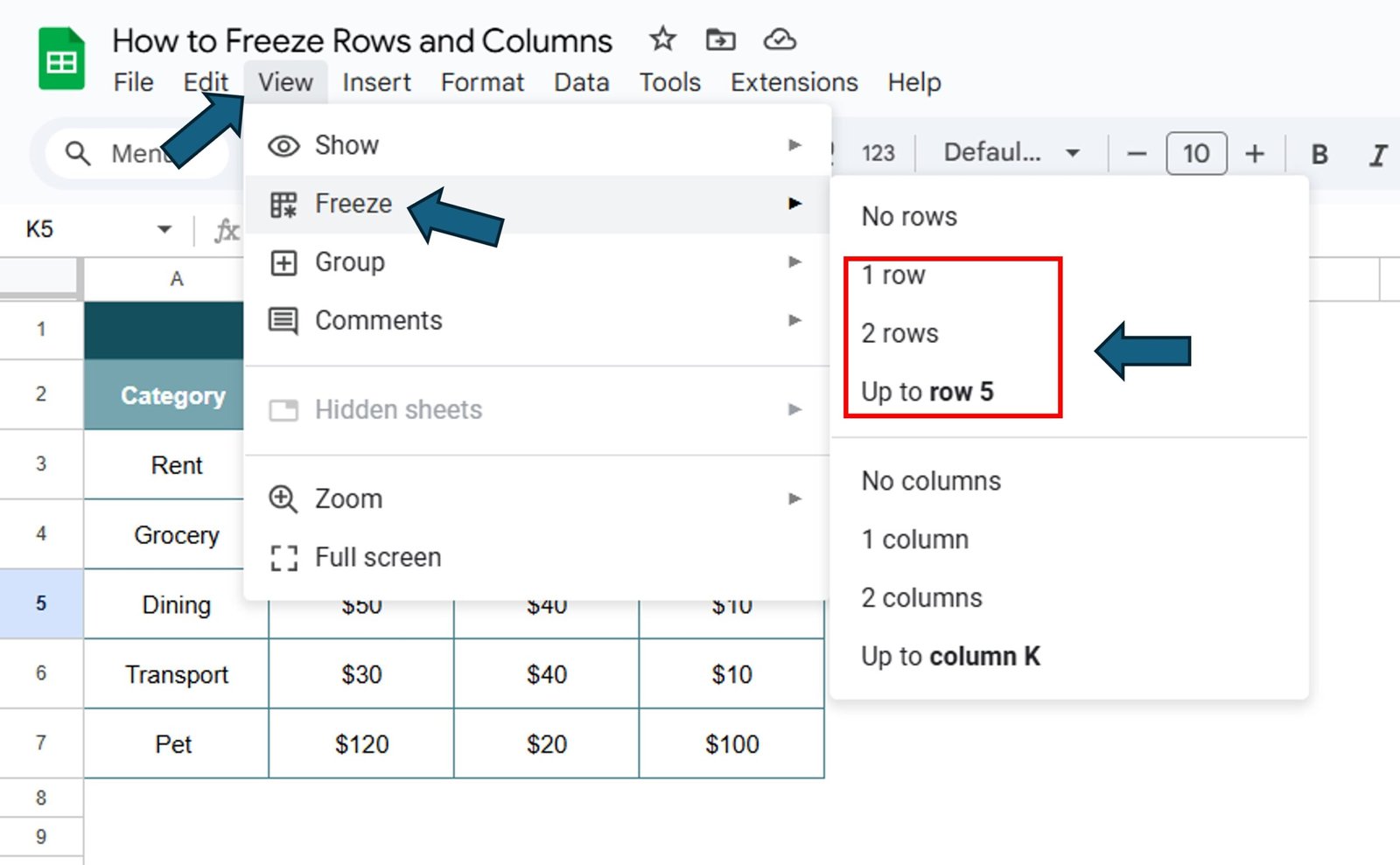
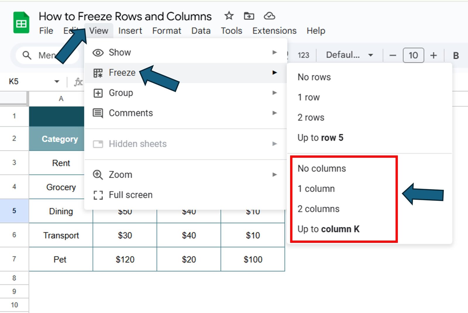
Go to the View Menu: Click on the “View” option in the top menu bar.
Choose “Freeze”: In the dropdown menu, hover over “Freeze” to see your options.
Select the Number of Rows to Freeze
Choose from:
- No rows: Unfreezes all rows.
- 1 row: Freezes the top row.
- 2 rows: Freezes the first two rows.
- Up to current row (X): Freezes all rows up to the selected row.
How to Freeze Columns in Google Sheets
Freezing columns is just as simple. Follow these steps:
- Open Your Google Sheet: Open the spreadsheet you want to edit.
- Select the Column to Freeze: Highlight the column you want to freeze, such as the first column for row labels.
- Go to the View Menu: Click on “View” in the top menu.
- Choose “Freeze”: Hover over “Freeze” in the dropdown menu.
Select the Number of Columns to Freeze
Choose from:
- No columns: Unfreezes all columns.
- 1 column: Freezes the first column.
- 2 columns: Freezes the first two columns.
- Up to current column (X): Freezes all columns up to the selected column.
Best Practices for Freezing Rows and Columns
To make the most of this feature, consider these tips:
- Freeze Only What’s Necessary: Freezing too many rows or columns can clutter your view. Stick to headers or key labels.
- Combine with Filters: Use filters alongside frozen headers to analyze your data efficiently.
- Test for Usability: Scroll through your spreadsheet after freezing to ensure it meets your needs.
- Use It for Collaboration: Freeze rows or columns that are essential for your team to understand the data structure.
Advantages of Freezing Rows and Columns
Freezing rows and columns provides several benefits:
- Improved Clarity: Keeps headers and labels visible at all times.
- Streamlined Data Entry: Makes it easier to enter data accurately without losing track of the context.
- Effortless Collaboration: Ensures that all users have a consistent view of the data structure.
Opportunities for Improvement in Freezing Rows and Columns
While freezing rows and columns is useful, there’s room for improvement:
- Freeze Multiple Sections: Allow users to freeze rows and columns at different positions, not just from the top or left.
- More Visual Cues: Highlight frozen sections more distinctly for better visibility.
- Enhanced Mobile Experience: Improve the freezing feature for mobile users to make it as seamless as the desktop version.
Frequently Asked Questions
1. Can I Freeze Both Rows and Columns at the Same Time?
Yes, you can freeze both rows and columns simultaneously. Just repeat the steps for freezing rows and columns separately.
2. How Do I Unfreeze Rows or Columns?
Go to View > Freeze and select No rows or No columns to unfreeze.
3. Does Freezing Work on Shared Sheets?
Yes, freezing rows and columns applies to all viewers of the shared sheet.
4. Can I Freeze Rows or Columns in the Middle of the Sheet?
No, freezing only works from the top or left edge of the sheet.
5. How Many Rows and Columns Can I Freeze?
You can freeze as many rows or columns as your sheet contains, up to the selected row or column.
Conclusion
Freezing rows and columns in Google Sheets is a simple yet powerful tool for improving your spreadsheet workflow. Whether you’re working on a large dataset, collaborating with a team, or simply trying to stay organized, this feature ensures critical information remains visible as you scroll. By following the steps and best practices in this guide, you’ll unlock the full potential of Google Sheets and make your data easier to manage.
Visit our YouTube channel to learn step-by-step video tutorials
Youtube.com/@NeotechNavigators
