Have you ever wondered how to quickly find the position of a specific item in a list? It might sound tricky, but thanks to Google Sheets‘ MATCH function, it’s easier than you might think! In this post, I’m going to walk you through how to use the MATCH Function in Google Sheets to find the position of an item in a list with an example. Plus, I’ll explain everything in simple, easy-to-understand language so you can follow along without any confusion!
What Is the MATCH Function in Google Sheets?
So, let’s start with the basics. The MATCH function is a super helpful tool in Google Sheets that searches for a value in a range of cells and then returns the position of that value in the list. Sounds useful, right?
Here’s the basic formula:
=MATCH(search_ key, range, [search_ type])
- search_ key: The value you’re trying to find.
- range: The cells where you’re searching.
- search_ type: This is optional. If you want an exact match, set this to “0.”
Now that you have an idea of what the MATCH function does, let’s dive into an example. Don’t worry if it sounds a bit technical — we’ll break it down step by step!
Example: How to Find an Employee’s Position Using Their ID
Imagine you have a list of employees with their ID numbers, names, and other details. You need to find out where a specific employee is in that list. Let’s see how the MATCH function can help!
The Data We’ll Use
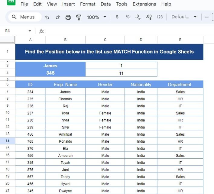
Here’s the list of employee information we’re working with:
Now, our goal is to find where the employee with the ID 345 appears in this list.

The Solution: Using the MATCH Function in Google Sheets
To find the position of the employee with ID 345, we’ll use the MATCH function. Here’s the formula:
=MATCH(345, A3:A22, 0)
Let me break it down for you:
345 is the employee ID we’re searching for.A3is the range of cells containing the ID numbers.
0 means we’re looking for an exact match.
When you run this formula, Google Sheets will return the number 11. This tells us that the employee with ID 345 (in this case, Toyah) is in the 11th position in our list. MATCH Function in Google Sheets
Why Should You Use the MATCH Function?
You might be thinking, “Why should I bother using the MATCH function?” Well, there are several great reasons!
- Quick Results: No more manually searching through large lists! The MATCH function finds the position instantly.
- Works With Other Formulas: You can combine MATCH with other functions, like INDEX, for even more powerful lookups.
- Time Saver: It’s a big time-saver when you’re dealing with dynamic data or need to find specific items often.
Wrapping Up: MATCH Function Made Easy
And there you have it! The MATCH function is a quick and simple way to find the position of any item in a list. It’s easy to use, and with just a little practice, you’ll be using it like a pro. Next time you need to search for something in a long list, give the MATCH function a try! MATCH Function in Google Sheets
Visit our YouTube channel to learn step-by-step video tutorials
Youtube.com/@NeotechNavigators
View this post on Instagram


