If you’ve ever wondered how to calculate the factorial of a number without doing all the multiplication yourself, you’re in the right place! In Google Sheets, the FACT Function in Google Sheets can do the heavy lifting for you, especially if you’re dealing with factorials for probabilities, statistics, or even math assignments. Don’t worry—this guide will break everything down in an easy-to-follow way, with plenty of examples to help you understand each step.
What Exactly is the FACT Function?
Before diving into examples, let’s quickly cover what the FACT function is all about. The FACT function in Google Sheets calculates the “factorial” of any non-negative whole number (like 1, 2, 3, and so on). In simple terms, a factorial means multiplying a number by every positive number below it. For example:
The factorial of 3 (written as 3!) is 3 x 2 x 1 = 6.
The factorial of 5 (5!) is 5 x 4 x 3 x 2 x 1 = 120.
If that sounds complex, don’t worry—it’s easier than you think once we get into some practical examples.
Why Would You Use Factorials?
Factorials might seem like something reserved for math class, but they’re actually quite useful in various situations. You’ll see them in probability calculations, combinatorics (like figuring out combinations and arrangements), and even some statistics. With the FACT function, you can skip the long multiplication steps and let Google Sheets give you the result in seconds.

How to Use the FACT Function in Google Sheets
Let’s go over the syntax first so you know what the FACT function looks like in Google Sheets. Don’t worry; it’s really straightforward!
=FACT(number)
Parts of the Formula:
- number: This is where you put the number you want to calculate the factorial for. Keep in mind, it has to be a whole number, and it can’t be negative.
Example: Calculating Factorials Step-by-Step
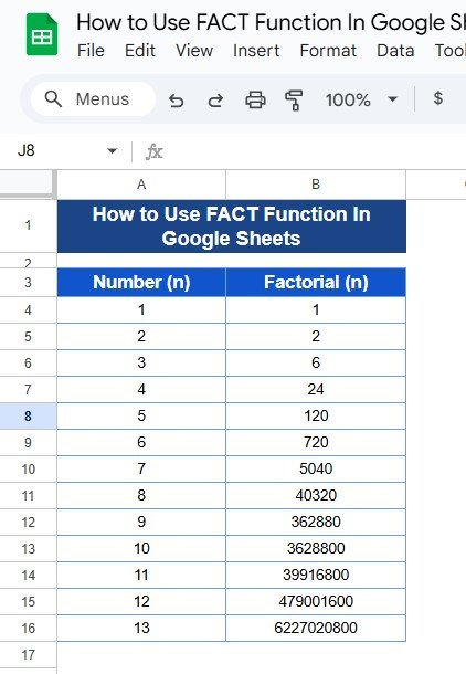
Let’s jump into an example to see exactly how this works in action. Here’s a list of numbers we’ll use for this example:
Step-by-Step Instructions for Using the FACT Function
- Select Your Cell: First, click on the cell where you want the factorial result to show up.
- Enter the Formula: In the formula bar, type =FACT(A4) (assuming cell A4 has your number). This formula will calculate the factorial of the number in cell A4.
Let’s take a closer look with a real example.
Example Calculation
Imagine you want to find the factorial of 4. Here’s what you would do:
Type the number 4 into cell A4.
In the next cell (say, B4), type =FACT(A4).
Press Enter, and the result—24—will appear. That’s because 4! (4 factorial) is 4 x 3 x 2 x 1, which equals 24.
You can do this for any number in the list, and Google Sheets will quickly give you the factorial in one easy step.
What the Result Table Looks Like
After you’ve set up the FACT function in Google Sheets, here’s the output you’ll get:

Pro Tips for Using the FACT Function
To make sure you get the most out of this function, here are a few tips to keep in mind:
- Stick to Whole Numbers: The FACT function works only with whole, positive numbers. If you enter a decimal, Google Sheets will round it down.
- Avoid Negatives: If you try to use a negative number, you’ll get an error because factorials aren’t defined for negative numbers.
- Watch Out for Big Results: Factorials get very large very quickly. For instance, 13! (the factorial of 13) is already over 6 billion! So be aware if you’re working with large numbers.
Wrapping Up: Why Use the FACT Function?
Using the FACT function in Google Sheets saves you from a lot of manual work and possible mistakes in calculating factorials. Instead of multiplying manually, you can let Google Sheets do the math for you. Next time you’re working on any math, statistics, or probability task that needs factorials, give this function a try!
Visit our YouTube channel to learn step-by-step video tutorials
Youtube.com/@NeotechNavigators
View this post on Instagram


