3 Powerful IF Function Tricks in Google Sheets

Google Sheets is a versatile tool for managing data, and one of its most powerful functions is the IF function. With IF functions, you can add logical decision-making capabilities to your spreadsheets. In this article, we’ll dive into 3 powerful IF function tricks in Google Sheets, complete with practical examples and step-by-step guidance.

These tricks will help you automate grading systems, analyze performance, and even determine eligibility for scholarships. By the end, you’ll be a pro at using IF functions to solve real-world problems!

Table of Contents

What is the IF Function in Google Sheets?

The IF function in Google Sheets is a logical formula that allows you to perform comparisons and return specific results based on a condition. The syntax of the IF function is:

=IF(condition, value_if_true, value_if_false)

Here’s what the components mean:

condition: The logical test (e.g., A1 > 50).

value_if_true: The value returned if the condition is true.

value_if_false: The value returned if the condition is false.

Now, let’s explore the 3 Powerful IF Function

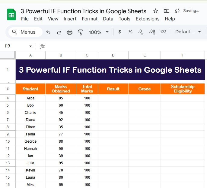
Example Data Setup

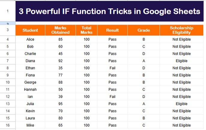
We’ll use the following dataset to demonstrate the three tricks:

Objective:

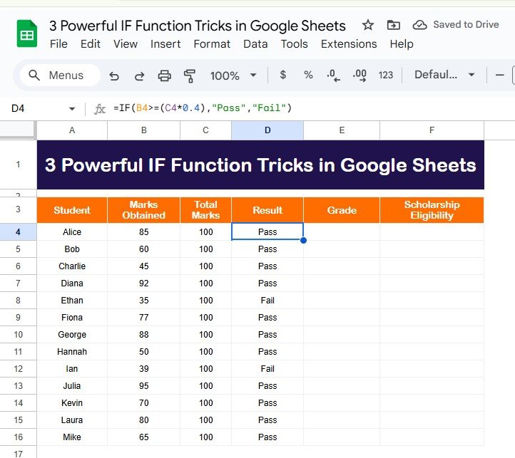
Determine whether each student has passed or failed based on their Marks Obtained. The passing criterion is 40% of the Total Marks.

Formula:

=IF(B2 >= (C2 * 0.4), “Pass”, “Fail”)

Explanation:

B2 refers to “Marks Obtained.”

C2 * 0.4 calculates 40% of the total marks.

If the marks obtained are greater than or equal to 40% of the total, the result is “Pass”; otherwise, it’s “Fail.”

Output:

Trick 2: Assigning Grades Using Nested IF

Objective:

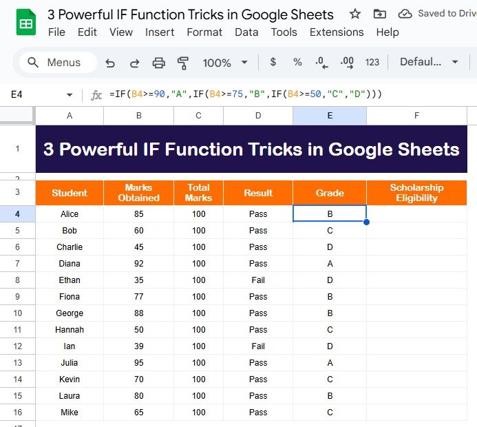
Assign grades to students based on their performance:

A: Marks ≥ 90
B: Marks ≥ 75
C: Marks ≥ 50
D: Marks < 50

Formula:

=IF(B2 >= 90, “A”, IF(B2 >= 75, “B”, IF(B2 >= 50, “C”, “D”)))

Explanation:

The formula uses nested IF functions to check multiple conditions.

The first condition (B2 >= 90) assigns “A.”

If the first condition is false, the formula moves to the next condition (B2 >= 75) and so on.

Output:

Trick 3: Scholarship Eligibility Using AND with IF

Objective:

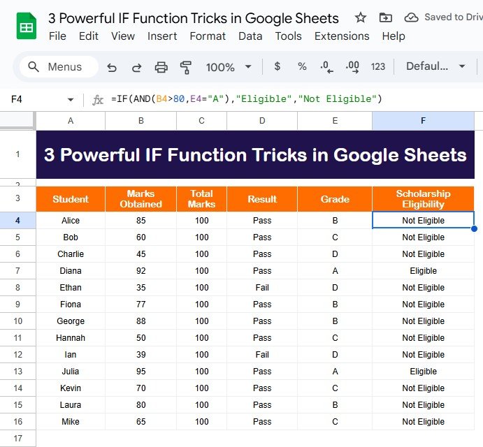
Determine scholarship eligibility. A student is eligible if:

Their grade is “A.”

Their marks are greater than 80.

Formula:

=IF(AND(B2 > 80, E2 = “A”), “Eligible”, “Not Eligible”)

Explanation:

The AND function evaluates multiple conditions:

B2 > 80: Marks must be greater than 80.

E2 = “A”: Grade must be “A.”

If both conditions are true, the result is “Eligible”; otherwise, it’s “Not Eligible.”

Output:

Advantages of Using IF Function Tricks

Automates Decision-Making: Save time by eliminating manual evaluations.
Handles Complex Logic: Use nested IF or logical functions like AND for advanced scenarios.
Improves Data Accuracy: Reduces human error in decision-based tasks.

Opportunities for Improvement in Using IF Functions

While the IF function is powerful, there are opportunities for improvement:

Performance on Large Data: Complex nested formulas can slow down large spreadsheets. Use alternatives like query functions or apps scripts for scalability.
Error Management: Include error-handling functions like IFERROR to avoid formula breaks.
Readability: Long nested formulas can become hard to read. Use helper columns to simplify.

Best Practices for Using IF Functions in Google Sheets

Simplify Logic: Avoid unnecessary nesting. Combine logical functions like AND/OR with IF.
Test Your Formulas: Use test data to ensure your formulas return the expected results.
Use Helper Columns: Break down complex formulas into smaller steps for clarity.

Conclusion

The IF function in Google Sheets is a powerful tool that can handle a variety of logical operations. By mastering the tricks we’ve covered—evaluating pass/fail, assigning grades, and determining scholarship eligibility—you can unlock the full potential of this function in your spreadsheets.