Google Sheets has a ton of amazing functions, but one that stands out when you want to convert numbers into characters is the UNICHAR Function in Google Sheets. It may sound a bit technical at first, but trust me, by the end of this guide, you’ll be using it like a pro! In this post, we’ll walk you through an easy-to-follow example of how the UNICHAR function works and why it can be so handy.
What is the UNICHAR Function?
First things first—what exactly is the UNICHAR function in Google Sheets? Essentially, the UNICHAR function allows you to return a character that corresponds to a given Unicode number. In simpler terms, if you input a number that represents a Unicode character, the function will give you the character that matches that number. This is super helpful when working with special characters or encoding.
The Formula: How to Use It
To break it down, here’s the syntax for the UNICHAR function:
=UNICHAR(number)
This formula takes a Unicode number as its input and returns the corresponding character. Now, let’s take a look at how this works with a real-world example.

Example: Convert Numbers to Alphabet Characters
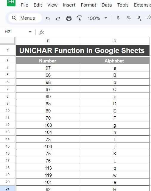
Let’s say we have a dataset in Google Sheets, like the one below, where we want to convert the numbers into their corresponding alphabet characters:
In column B, we have numbers, and we want to use the UNICHAR function to get the characters for each number in column C. Here’s the formula you’ll use in cell C3:
=UNICHAR(B3)
You can drag this formula down to fill all the cells in column C.
How Does It Work?
When you type =UNICHAR(B3) into your cell, Google Sheets takes the Unicode number from cell B3 (which is 97 in this case) and converts it into the corresponding character, which is the letter ‘a’. Cool, right?
Results: Here’s What You’ll See
After applying the formula, here’s the output you will get in column C:
Number Alphabet
As you can see, the UNICHAR function has successfully converted the numbers into their corresponding Unicode characters. This function can return characters like letters, special symbols, or even emojis if you use the right number!
Why Use UNICHAR in Google Sheets?
Now you might be wondering, why would I even need to use the UNICHAR function? Well, here are a few reasons why it’s a hidden gem:
- Data Transformation: Quickly convert numeric data into characters or symbols.
- Special Symbols: Easily insert special Unicode characters into your dataset without memorizing complex codes.
- Efficiency: Automate character generation for large datasets, saving tons of time.

Conclusion
The UNICHAR function may not be one of the most talked-about functions in Google Sheets, but it is definitely one of the most useful when it comes to working with Unicode characters. Whether you’re transforming data, adding special symbols, or just want to explore the full range of characters, this function can be your go-to tool.
Visit our YouTube channel to learn step-by-step video tutorials
Youtube.com/@NeotechNavigators
View this post on Instagram


