A dynamic calendar with holidays and events in Google Sheets redraws all twelve months the moment you pick a different year, and automatically colours every date that appears in your holiday and event list. You build it once and reuse it every year, with no copying of month grids and no manual colouring.
This tutorial is for anyone who plans in Google Sheets: office admins, teachers, small business owners and families. I will show you the finished calendar, then explain the formulas behind it: DATE, WEEKDAY, SEQUENCE and LET to build each month, a data-validation dropdown for the year, and COUNTIF inside conditional formatting to highlight holidays.
🎥 Watch the Video Tutorial
Get the ready-made Holiday and Event Calendar
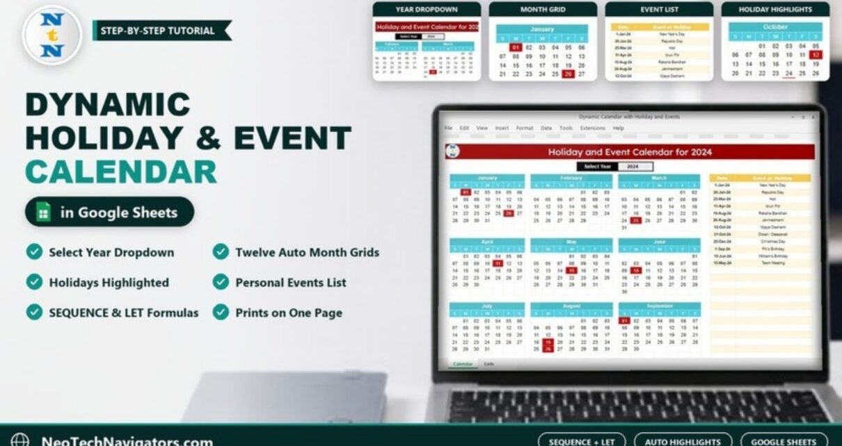
What the Finished Calendar Looks Like

- Title that updates with the year: “Holiday and Event Calendar for 2024”.
- Select Year dropdown under the title.
- Twelve month grids laid out in four rows of three, each with Sunday-to-Saturday columns (S M T W T F S) and two-digit day numbers (01, 02 …).
- Date / Event or Holiday list on the right. In the sample it holds entries such as 1-Jan-24 New Year’s Day, 26-Jan-24 Republic Day, 25-Mar-24 Holi, 31-Oct-24 Diwali / Deepavali and 25-Dec-24 Christmas Day, plus personal items like birthdays and a team meeting.
- Dark red highlight on every calendar date found in that list.
The calendar fits one landscape page, so it prints cleanly or can be saved as a PDF.
Functions Used and What Each Argument Means
| Function | Syntax | Role in the calendar |
|---|---|---|
| DATE | DATE(year, month, day) | Builds the first day of each month from the selected year |
| WEEKDAY | WEEKDAY(date, [type]) | Returns 1 (Sunday) to 7 (Saturday) with type 1, so you know how far to step back to the Sunday |
| SEQUENCE | SEQUENCE(rows, columns, start, step) | Generates the 6 × 7 grid of consecutive dates |
| LET | LET(name, value, …, calculation) | Stores intermediate values so the formula stays readable |
| MONTH | MONTH(date) | Checks whether a grid date belongs to the month being displayed |
| COUNTIF | COUNTIF(range, criterion) | Tests whether a calendar date exists in the holiday list |
Step-by-Step: Build the Dynamic Calendar
Step 1: Create the year dropdown
Put a list of years somewhere out of the way, for example on a sheet called Lists, cell A1:
=SEQUENCE(31, 1, 2020)This returns 2020 to 2050. Select the year cell on the calendar (in this example C2), open Data > Data validation > Add rule, choose Dropdown (from a range) and point it at Lists!A1:A31. To support more years later, just extend the list.
Step 2: Make the title dynamic
="Holiday and Event Calendar for " & C2Step 3: Build one month grid
Type the weekday headers S, M, T, W, T, F, S in one row. In the first cell beneath them, enter this formula for January (month 1):
=ARRAYFORMULA(LET(
  first, DATE($C$2, 1, 1),
  start, first - WEEKDAY(first) + 1,
  d,     SEQUENCE(6, 7, start),
  IF(MONTH(d) = 1, d, "")
))
It finds the 1st of the month, steps back to the Sunday on or before it, fills 42 consecutive dates (six weeks), and blanks out any date that belongs to the previous or next month.
Select the grid and apply Format > Number > Custom number format with dd so each cell shows 01, 02, 03 instead of a full date.
Step 4: Copy for the other eleven months
Copy the block and change the two month numbers (the 1 inside DATE and the 1 in MONTH(d) = 1) to 2 for February, 3 for March, and so on up to 12.
Step 5: Add the holiday and event list
Create two columns headed Date and Event or Holiday (for example in AB4:AC40). Enter real dates, not text, and a short name for each.
Step 6: Highlight holidays with conditional formatting
Select all twelve grids, open Format > Conditional formatting, choose Custom formula is and enter (where B5 is the top-left cell of your selection):
=AND(B5 <> "", COUNTIF($AB$4:$AB$40, B5) > 0)Set a dark red fill and white text, then click Done.
Worked Example: January 2024
Select 2024 in the year cell. The formula then calculates:
first = DATE(2024, 1, 1)        → Monday 1 Jan 2024
WEEKDAY(first)                  → 2
start = 1 Jan 2024 - 2 + 1      → Sunday 31 Dec 2023
The first grid row therefore contains 31 Dec 2023 (blanked because it is not January), then 01 to 06 under M to S. That is exactly what the January grid in the screenshot shows. Because 1-Jan-24 and 26-Jan-24 are in the list, the conditional-format rule turns those two cells dark red. Switch the dropdown to 2025 and every grid and highlight recalculates.
Useful Variations
1. Start weeks on Monday
start, first - WEEKDAY(first, 2) + 1Change the headers to M T W T F S S to match.
2. Highlight today
Add a second conditional-format rule with a different colour:
=B5 = TODAY()3. Shade weekends
=AND(B5 <> "", WEEKDAY(B5) = 1)Use 1 for Sunday; add OR(WEEKDAY(B5)=1, WEEKDAY(B5)=7) to include Saturday.
4. Repeat birthdays every year
Birthdays fall on the same day each year, so match month and day rather than the full date (keep these in a separate range, here AE4:AE40):
=AND(B5 <> "", SUMPRODUCT(($AE$4:$AE$40 <> "") * (MONTH($AE$4:$AE$40) = MONTH(B5)) * (DAY($AE$4:$AE$40) = DAY(B5))) > 0)The $AE$4:$AE$40 <> "" part matters: Google Sheets reads an empty cell as day zero (30 Dec 1899), so without it every 30 December would be highlighted. Festivals such as Holi or Diwali move each year, so keep them as full dates in the main list.
5. Count events in a month
=COUNTIFS($AB$4:$AB$40, ">=" & DATE($C$2, 1, 1), $AB$4:$AB$40, "<=" & EOMONTH(DATE($C$2, 1, 1), 0))Place it beside a month name to show how many listed items fall in that month.
Common Errors and Fixes
| Problem | Cause | Fix |
|---|---|---|
| #REF! “Array result was not expanded” | Something is typed inside the 6 × 7 area | Clear the cells the grid needs |
| Grid shows numbers like 45292 | Cells are not formatted as dates | Apply the custom format dd |
| Every blank cell turns red | COUNTIF matches empty list rows | Keep the B5 <> "" check in the rule |
| A holiday is not highlighted | Date was typed as text or for the wrong year | Re-enter as a date; check the year matches the selection |
| Days sit under the wrong weekday | WEEKDAY type does not match headers | Use type 1 for Sunday start, type 2 for Monday start |
Tips for Printing and Sharing
- Use File > Print, choose Landscape and Fit to width for a one-page wall calendar.
- Use File > Download > PDF to send it by email.
- Share with Viewer access if colleagues only need to read it; give editors access only to the event list.
- Keep holidays and personal events in the same list but name them clearly, as in the sample (“PK’s Birthday”, “Team Meeting”).
Related Calendars and Guides
For a shorter walkthrough of the grid technique, see 6 easy steps to a dynamic calendar in Google Sheets. If you need calendars for a specific job, the Holiday Schedule Calendar in Google Sheets, Annual Leave Calendar, Event Planning Calendar and Academic Year Calendar build on the same ideas.
If you want to go further with structured lessons on date, lookup and logical formulas, the 100 formulas course on NextGenTemplates Academy covers them step by step; the logic carries straight over to Google Sheets.
Frequently Asked Questions
How do I change the year on the calendar?
Choose a different year in the Select Year dropdown. All twelve month grids, the title and the highlights update immediately.
Can I add my own events and birthdays?
Yes. Add a row to the Date / Event or Holiday list with a real date. If the date is in the selected year, it is highlighted automatically.
Why do some months need six rows?
A month that starts late in the week and has 30 or 31 days can spill into a sixth week, so every grid reserves six rows. March and June 2024 in the screenshot both use the sixth row.
Can the calendar sync with Google Calendar?
Not by itself. It is a spreadsheet view of your list. Syncing would need Apps Script or an add-on.
Will it work for any country’s holidays?
Yes. The calendar only highlights the dates you enter, so you can list holidays for India, the US, the UK or anywhere else.
Does it work in Excel?
The same approach works in Excel 365, which also has SEQUENCE and LET; only the dropdown and conditional-formatting menus differ.
Wrapping Up
With one year dropdown, one SEQUENCE formula per month and a single conditional-formatting rule, you get a calendar that rebuilds itself every year and highlights every holiday and event you list. Build it once using the steps above, or start from the ready-made template if you would rather skip the setup.
Get the Dynamic Holiday and Event Calendar in Google Sheets
📅 Last updated: October 2026