If you’ve ever found yourself wondering how to search for data in Google Sheets with more flexibility, then you’re in the right place! In this guide, I’ll walk you through a powerful combination of two functions—VLOOKUP with MATCH Function—which together make data searching a breeze.
But before diving in, let’s think about why this combination is so useful.
Why Use VLOOKUP with MATCH?
We all love VLOOKUP, but sometimes it can feel a bit restrictive. For example, when you’re looking for a value based on a subject in one column but want the flexibility to change the column you’re pulling from, MATCH comes to the rescue! Instead of hardcoding the column index in your VLOOKUP formula, you can dynamically set it using MATCH, which makes your formula even more adaptable.
Now, let’s move on to the fun part—learning how to use it with an example!
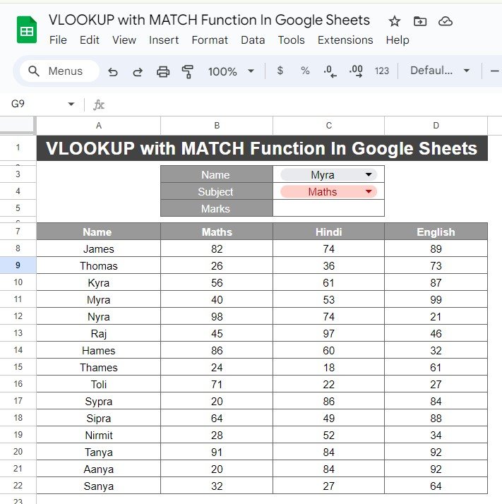
Imagine you want to know Myra’s score in Maths. We will be using VLOOKUP with MATCH to get this value.

Setting Up the Formula
Here’s how the formula looks:
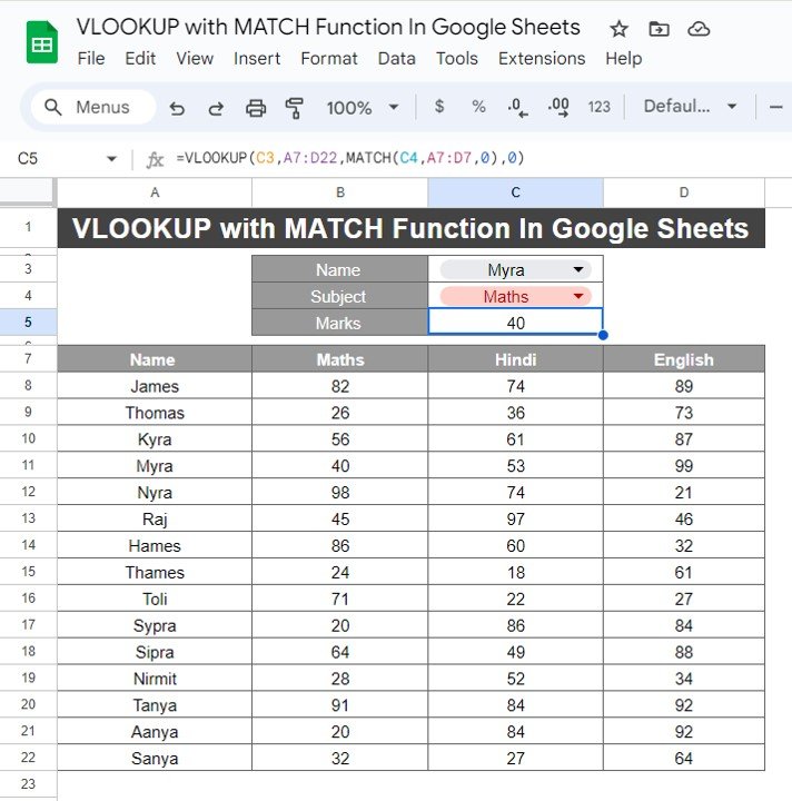
=VLOOKUP(C3,A7:D22,MATCH(C4,A7:D7,0),0)
Let’s break it down step by step, so you can understand how it works:
- VLOOKUP(C3, A7, …): The VLOOKUP function is searching for the value in cell C3 (which is “Myra”) in the range A7.
- MATCH(C4, A7, 0): The MATCH function helps to locate the exact column to pull the data from. Here, it’s looking for the value in C4 (which is “Maths”) within the header row A7. It returns the position of “Maths” in that row, which is column 2.
The final 0 is for an exact match.
In simple terms, we’re telling Google Sheets: “Find Myra in the first column, and based on the subject ‘Maths,’ return the score.”
The Result
After applying the formula, you’ll get the following output:

Why This Formula Works So Well
- Dynamic Column Selection: By using MATCH, you make your formula more dynamic, allowing you to change the column you pull data from without manually editing the formula every time.
- Saves Time: Instead of writing separate formulas for different subjects or fields, you can use a single formula that adjusts based on what you input.
- Improved Accuracy: The exact match logic ensures you get precise results every time, reducing errors.
Final Thoughts
Combining VLOOKUP with MATCH in Google Sheets gives you an extra layer of flexibility. Whether you’re dealing with a small dataset or a large one, this formula helps streamline the process of looking up data across different columns, and best of all, it’s easy to implement once you get the hang of it.
Visit our YouTube channel to learn step-by-step video tutorials
Youtube.com/@NeotechNavigators


