Every month the owner of Lone Star Landscaping asks the same thing: are we over budget? Receipts pile up in one long list, a typo in a category quietly drops a $160 receipt from the totals, and nobody can see which category ate the budget. This business expense tracker in Google Sheets fixes it with a category dropdown that rejects typos, one SUMIFS formula for the whole monthly summary, red, amber and green budget status, four KPI cards and a spend vs budget chart. The free practice file has 176 made-up expenses for July to October and a $17,000 monthly budget. Built-in features only, no add-ons.
📥 Download the FREE Practice File (Excel .xlsx)
Same tabs as the video: README, Practice, Solution, Lists
📄 Make Your Own Copy in Google Sheets
Opens a copy in your Google Drive – sign in to Google first
Watch the Video Tutorial
Video Overview
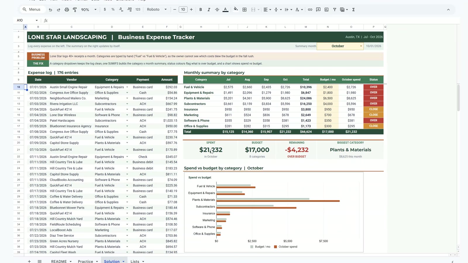
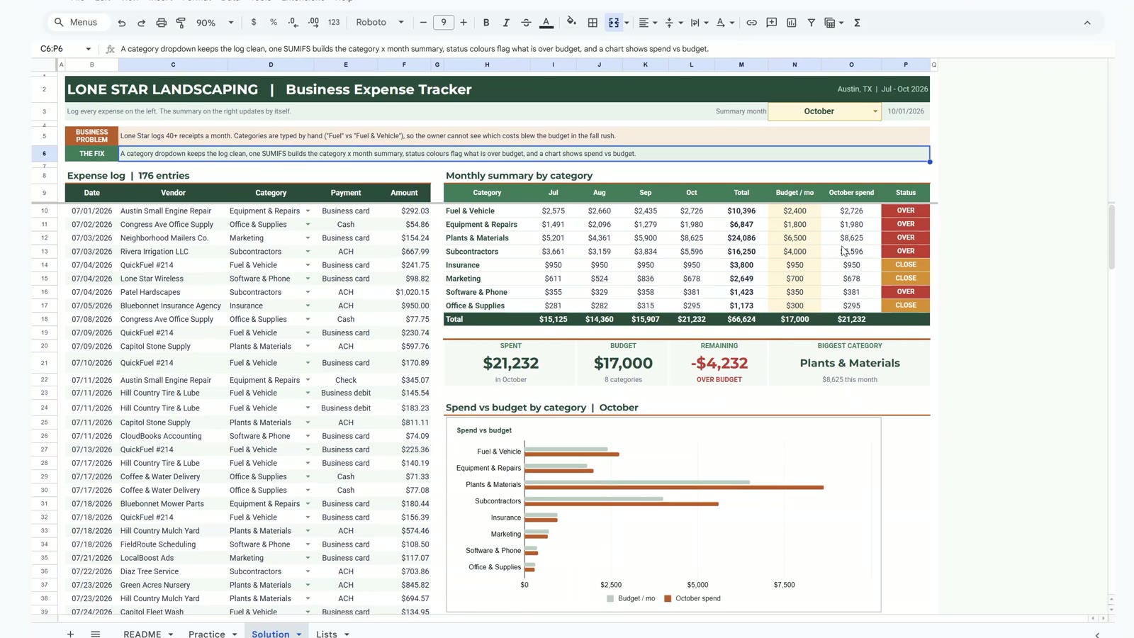
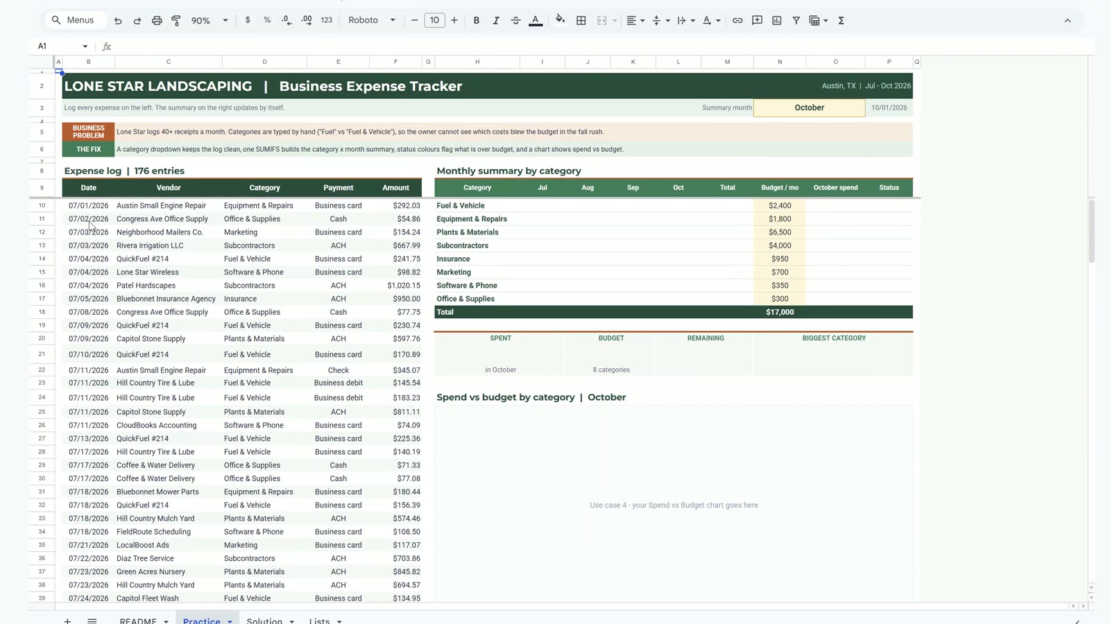
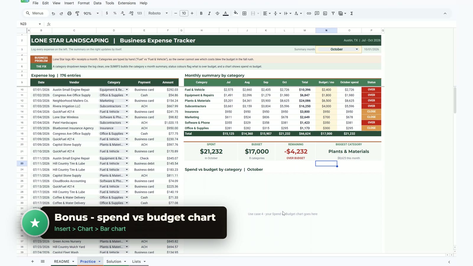
The video starts with the finished tracker: October is $4,232 over budget and the card is red, then switching the summary month to August shows $2,640 under budget in green. After a tour of the practice file (README, Practice, Solution and Lists sheets) you build three steps and a bonus chart, about 15 minutes in total. Pause anywhere and build it along with the practice file.
What You Will Build
- A category dropdown that rejects any category that is not on the list.
- A category by month table filled by one SUMIFS formula (8 categories x 4 months = 32 cells).
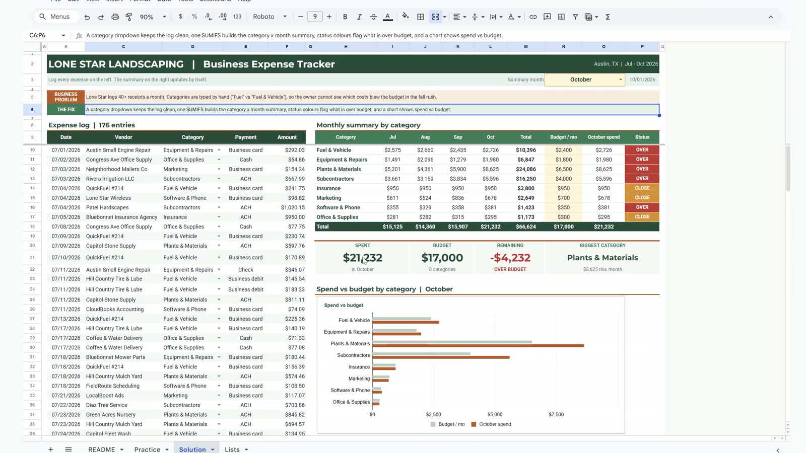
- A summary month picker with OVER, CLOSE and OK status colours and four KPI cards: spent, budget, remaining and biggest category.
- A bonus bar chart of spend against budget that follows the month you pick.
The Problem: A Business Expense Tracker in Google Sheets That Lies
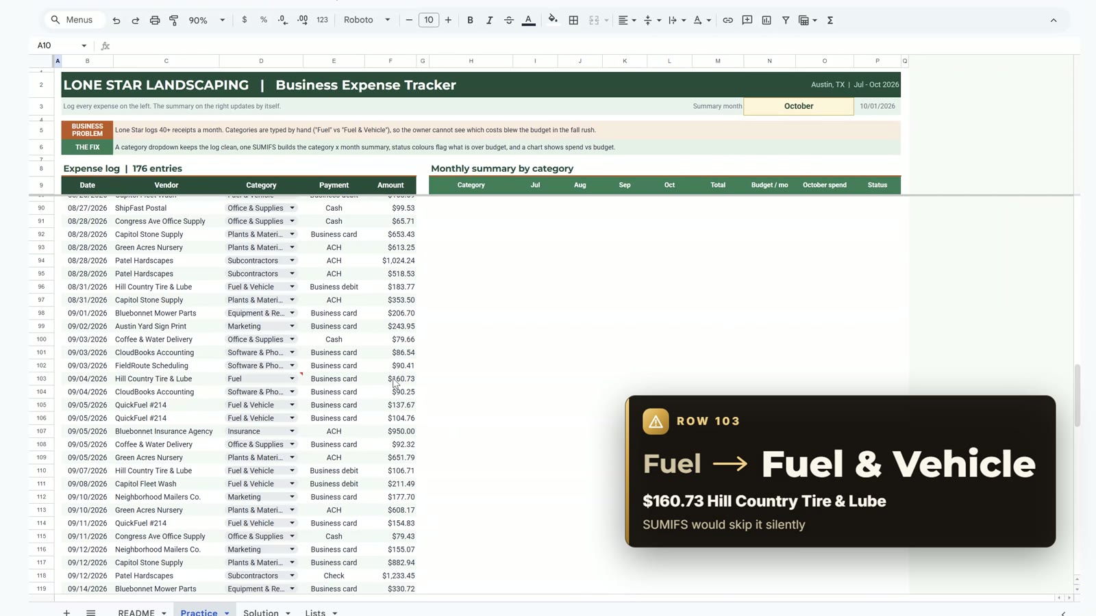
Lone Star Landscaping in Austin, Texas logs about 40 receipts a month across eight categories. Categories are typed by hand, so the owner cannot tell which one is draining the budget, and a misspelled category is silently left out of every total. Row 103 in the practice file is a real example: a $160.73 receipt from Hill Country Tire & Lube was typed as Fuel instead of Fuel & Vehicle.
Step 1: A Category Dropdown That Catches Typos
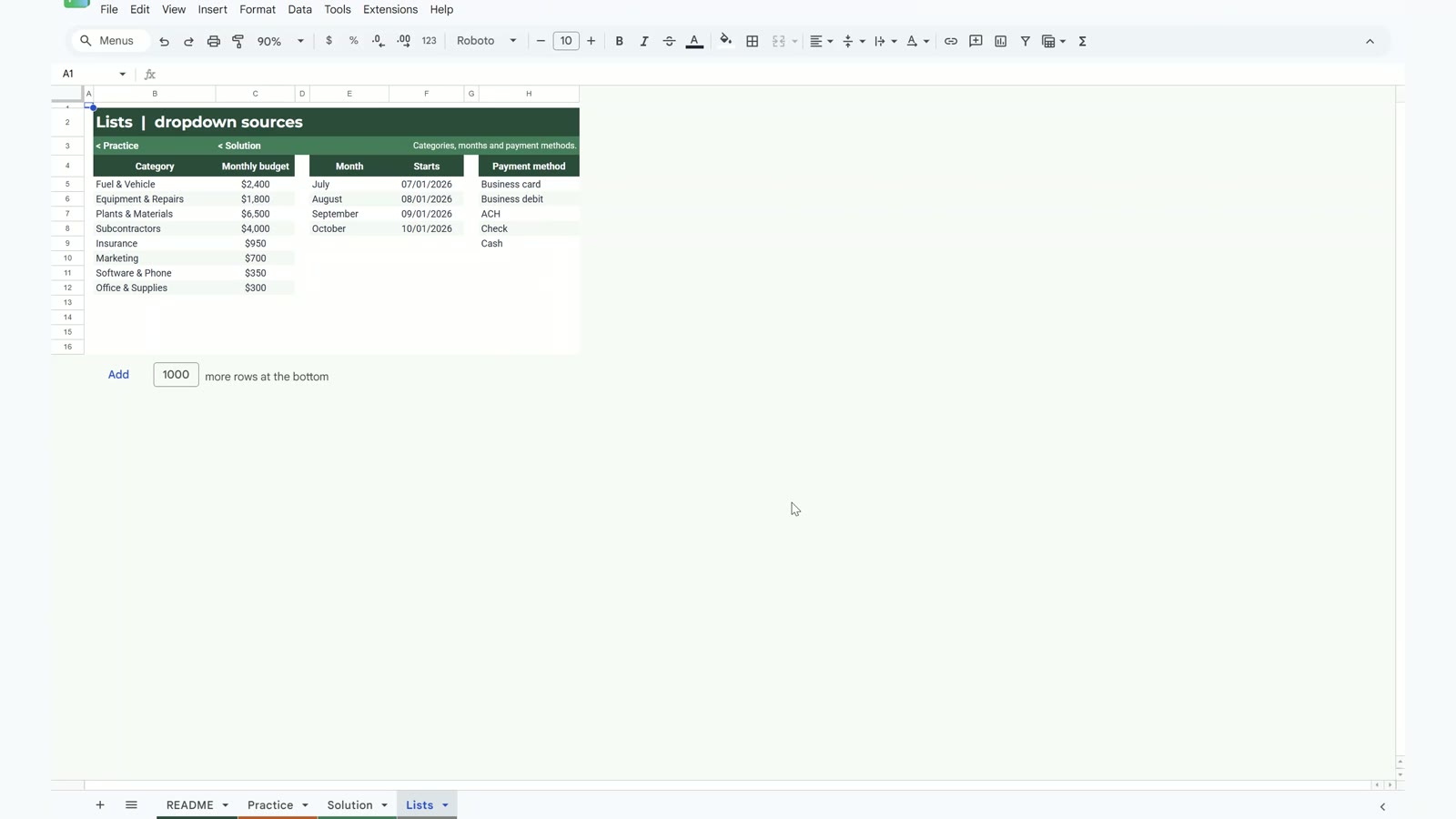
Select the Category column (D10 to D185), choose Data, then Data validation, then Add rule. Under criteria choose Dropdown (from a range) and type Lists!B5:B12, the eight category names. Open Advanced options and set invalid data to Reject the input. Every cell is now a dropdown.
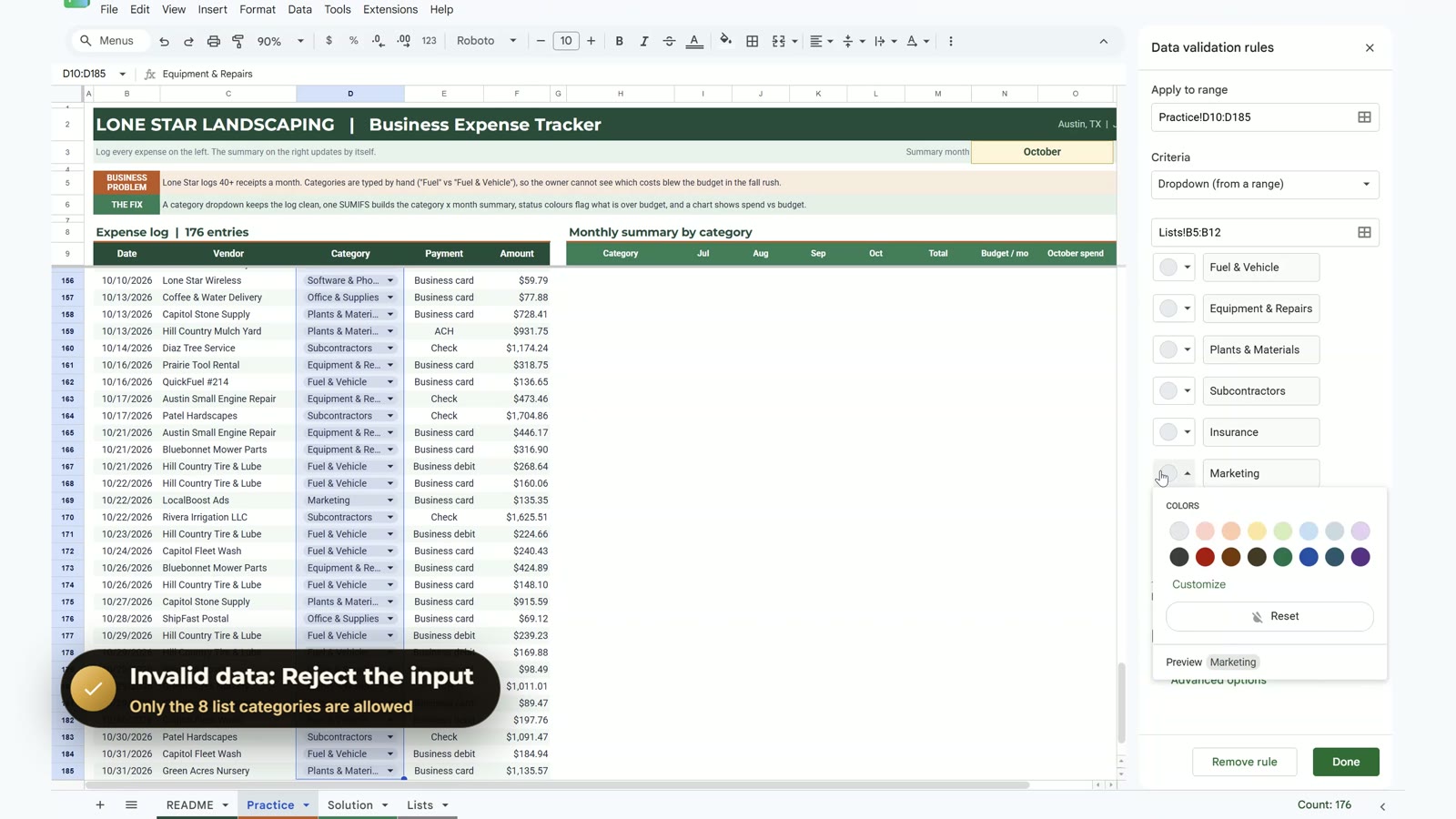
Scroll to row 103 and you will see a red mark in the corner: the category says Fuel, which is not on the list. Pick Fuel & Vehicle from the dropdown in D103 and the mark disappears. A SUMIFS looking for Fuel & Vehicle would have skipped that $160.73 without any error.
Step 2: One SUMIFS for the Whole Monthly Summary
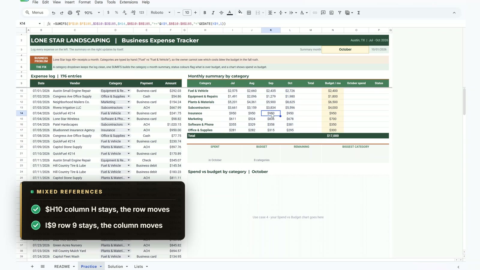
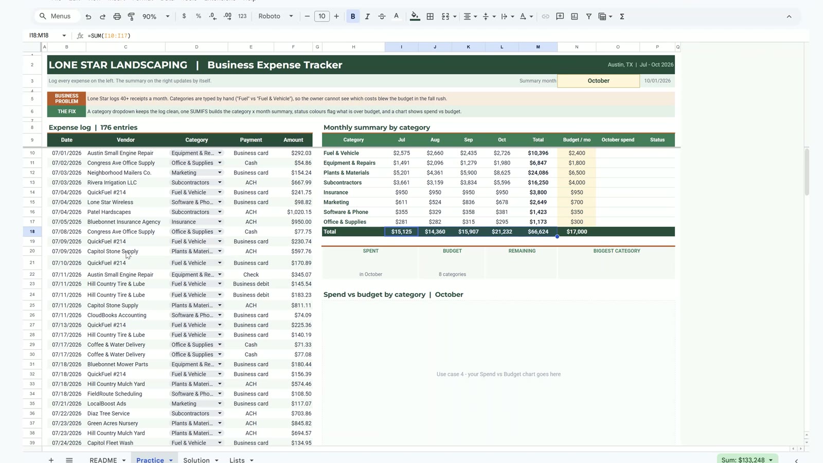
In I10 (Fuel & Vehicle, July) type this formula. Press F4 to add the dollar signs: lock the sum range and the two criteria ranges completely, put the dollar sign only before the H in $H10 and only before the 9 in I$9.
=SUMIFS($F$10:$F$185,$D$10:$D$185,$H10,$B$10:$B$185,">="&I$9,$B$10:$B$185,"<"&EDATE(I$9,1))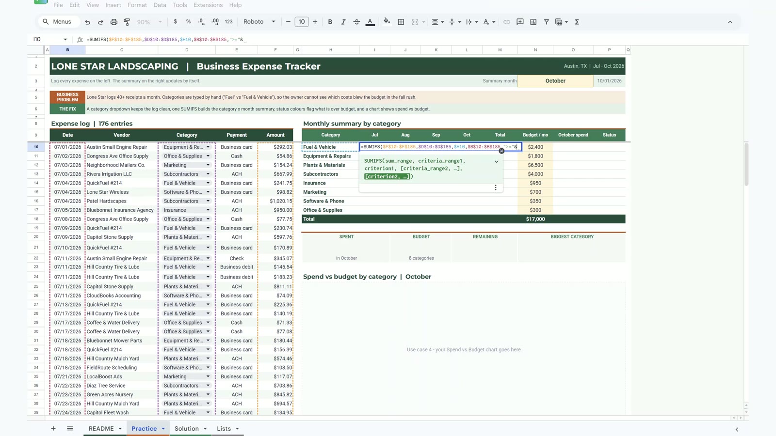
The month headers in row 9 look like text but each one is a real date, the first day of the month, only formatted as mmm. EDATE(I$9,1) moves forward by one month, so the formula adds every receipt dated on or after July 1 and before August 1. The first result is $2,575.
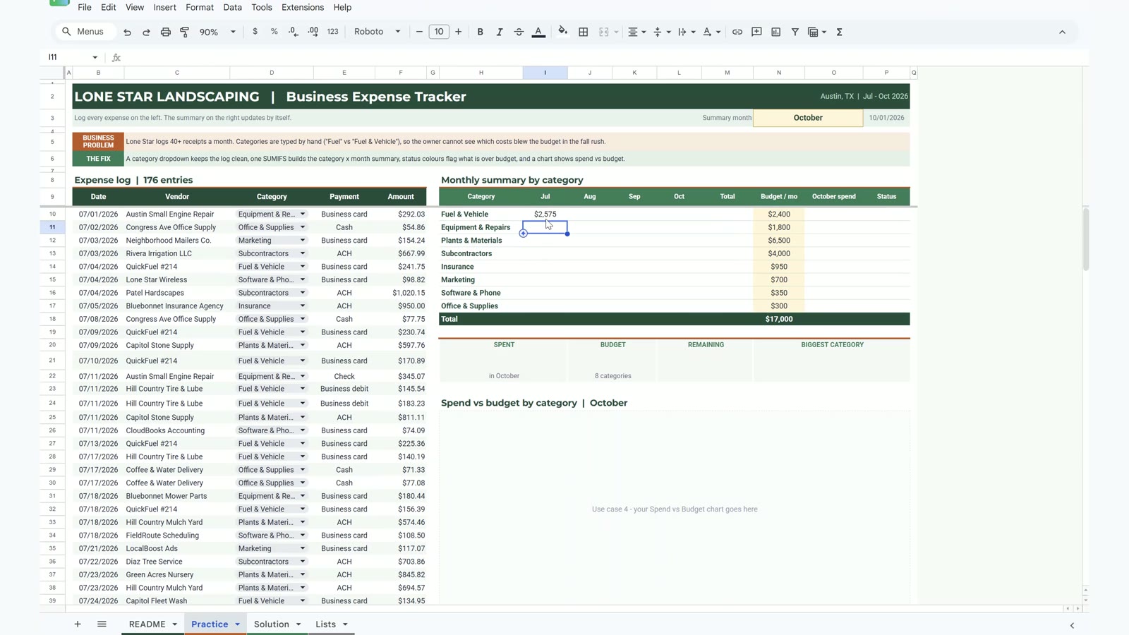
Copy I10, select I10 to L17 and paste. The mixed references make one formula correct for all 32 cells. Then add the totals: =SUM(I10:L10) in M10 copied down, and =SUM(I10:I17) in I18 copied across. The grand total is $66,624, every one of the 176 receipts.
Step 3: Summary Month, Budget Status and Cards
Select N3 (the yellow cell) and add a dropdown from the range Lists!E5:E8, the four month names. P3 already holds an XLOOKUP that turns the month name into its start date. In O10 use the same SUMIFS, but with P3 instead of I9, then copy it to O17 and add =SUM(O10:O17) in O18.
=SUMIFS($F$10:$F$185,$D$10:$D$185,$H10,$B$10:$B$185,">="&$P$3,$B$10:$B$185,"<"&EDATE($P$3,1))Then the status in P10, copied down to P17:
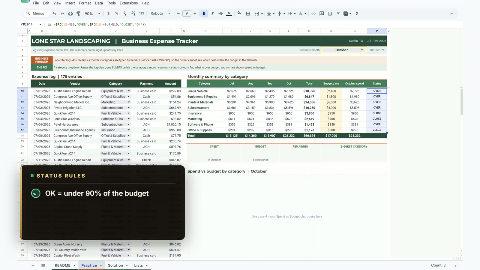
=IF(O10>N10,"OVER",IF(O10>=0.9*N10,"CLOSE","OK"))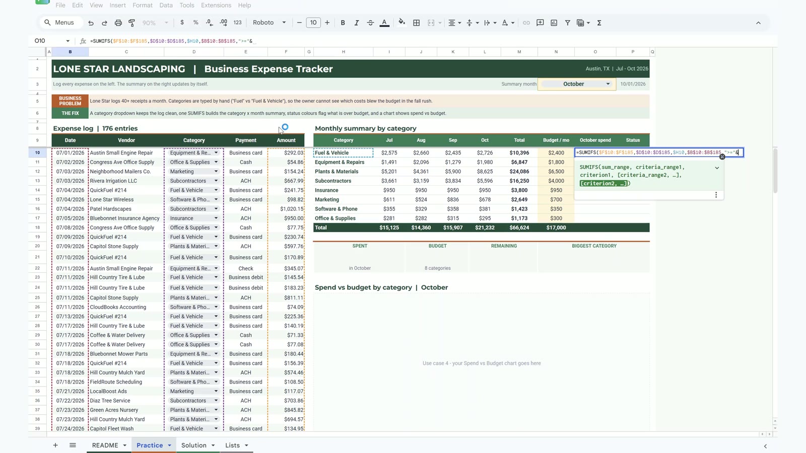
Select P10 to P17 and open Format, then Conditional formatting. Add three rules: text is exactly OVER (red fill, white text), CLOSE (amber) and OK (green). Insurance shows CLOSE every month because it is a fixed bill of exactly $950.
The four cards: Spent is =O18, Budget is =N18, Remaining is =N18-O18 (negative turns red) with =IF(L21<0,"OVER BUDGET","UNDER BUDGET") below it. The Biggest category card uses INDEX and MATCH:
=INDEX(H10:H17,MATCH(MAX(O10:O17),O10:O17,0))=TEXT(MAX(O10:O17),"$#,##0")&" this month"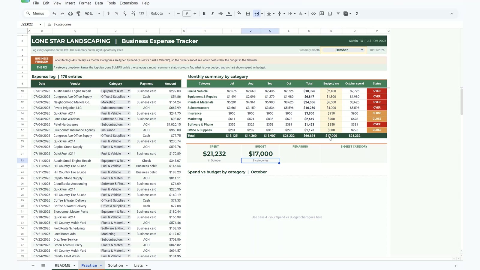
Bonus: Spend vs Budget Chart
Select the category names (H9 to H17), hold Control and also select N9 to O17 (budget and month spend). Choose Insert, then Chart, pick the bar chart, set the budget series to light green and the spend series to dark orange, put the legend at the bottom and title it Spend vs budget. Move it over the empty box and resize it. Every orange bar that runs past its green bar is a category over budget.
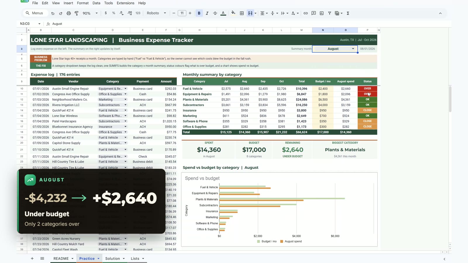
Flip through the months: Fuel & Vehicle is over budget in every single month, so the budget itself is too low and the owner should raise it.
Use This Business Expense Tracker in Google Sheets for Your Own Company
Change the categories and budgets on the Lists sheet, type your own expenses in the log and add new rows inside the log, above the last row, so every formula range grows with it. If you get stuck, compare with the Solution sheet in the practice file.
📥 Download the FREE Practice File (Excel .xlsx)
Same tabs as the video: README, Practice, Solution, Lists
📄 Make Your Own Copy in Google Sheets
Opens a copy in your Google Drive – sign in to Google first
Want Income Tracking Too?
For a ready-made version that tracks income as well as expenses, look at the Income and Expense Dashboard in Google Sheets from Next Gen Templates. Also work in Excel? The Excel Pivot Tables & Dashboards: Basic to Advanced course teaches dashboards step by step.
🛒 Get the Income and Expense Dashboard
Google Sheets · tracks income too · Next Gen Templates
Frequently Asked Questions
How do I make a business expense tracker in Google Sheets?
Keep one row per receipt (date, vendor, category, payment, amount), add a category dropdown so every row uses the same spelling, then use one SUMIFS formula to total each category by month. A budget column, a status formula and a few KPI cards turn the log into a monthly summary. The video builds all of this step by step.
Why use a dropdown for the category?
SUMIFS only matches text that is exactly the same. One receipt typed as Fuel instead of Fuel & Vehicle is silently skipped and the total comes out too low, with no error. A dropdown from a range with Reject the input stops the typo before it happens.
Why does SUMIFS use start and end dates instead of the MONTH function?
July of this year and July of next year are both month 7, so MONTH would add them together. Comparing the date with >= the first day of the month and < EDATE(first day, 1) always picks one exact month and year, so the sheet keeps working when you add next year's expenses.
What does the ampersand do in ">="&I$9?
It joins the operator to the real date in the cell. If you type ">=I9" all inside the quotes, Google Sheets compares against the text I9 and the result is zero.
What do $H10 and I$9 mean?
They are mixed references. $H10 keeps the formula on column H (the category) while the row changes, and I$9 keeps it on row 9 (the month) while the column changes, so one formula fills all 32 cells.
How are OVER, CLOSE and OK decided?
OVER means the month's spend is above the budget. CLOSE means it is at least 90% of the budget. Anything else is OK. Conditional formatting colours the three words red, amber and green.
Can I use this tracker for my own business?
Yes. Change the categories and monthly budgets on the Lists sheet, type your own expenses in the log and add new rows inside the log (above the last row) so every formula range grows with it.
More Google Sheets tutorials are on the NeoTech Navigators blog and the YouTube playlist.