Magic Search Box in Google Sheets with FILTER Formula

A magic search box in Google Sheets lets you pick a column from a dropdown, type a keyword, and instantly see only the matching rows, with totals at the top that update for the result. It works with one formula built from FILTER, CHOOSECOLS, MATCH, LEFT, LEN and IFERROR, so there are no scripts or add-ons to install.

This tutorial uses a sales dataset as the example. You will learn the formula argument by argument, see a worked example with the real numbers from the template, and get practical variations such as “contains” search, case-sensitive search and searching across two fields.

🎥 Watch the Video Tutorial

Open the Free Practice File

How the Template Is Set Up

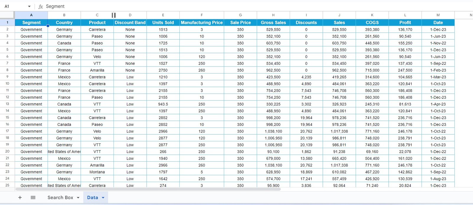
The file has two tabs: Data and Search Box.

The Data tab

The Data tab holds the raw sales records in columns A to M: Segment, Country, Product, Discount Band, Units Sold, Manufacturing Price, Sale Price, Gross Sales, Discounts, Sales, COGS, Profit and Date. The formula reads rows 2 to 701.

Data tab with sales records: Segment, Country, Product, Discount Band, Units Sold, Gross Sales, COGS, Profit and Date — The Data tab: the source table the search box filters

The Search Box tab

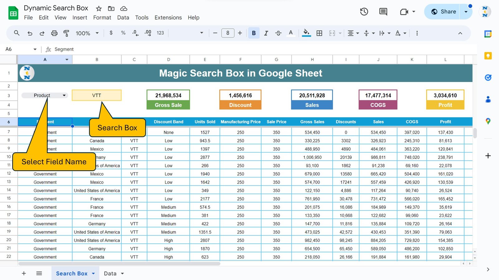
A3 – field dropdown: choose which column to search, for example Product.
B3 – search box: the yellow cell where you type the keyword.
Totals cards: Gross Sale, Discount, Sales, COGS and Profit for the filtered rows.
Row 6 – headers: the same column headers as the Data tab. The result starts below them in row 7.

Search Box tab with Product selected in A3 and VTT typed in B3, showing totals cards and only VTT rows — Search Box tab: field name in A3, keyword in B3, matching rows below

The Magic Search Box Formula

This formula sits in cell A7 of the Search Box tab and spills the matching rows:

=IFERROR(FILTER(Data!A2:M701, LEFT(CHOOSECOLS(Data!A2:M701, MATCH(A3, 6:6, 0)), LEN(B3)) = B3), "No Data Available")

Syntax breakdown

Part	What it means
`Data!A2:M701`	The full data range to return (all 13 columns)
`MATCH(A3, 6:6, 0)`	Finds the position of the chosen field name in header row 6, e.g. Product = 3
`CHOOSECOLS(range, n)`	Picks only that column from the data, e.g. the Product column
`LEN(B3)`	Counts the characters typed in the search box
`LEFT(column, LEN(B3)) = B3`	Keeps rows whose value starts with the typed keyword
`FILTER(range, condition)`	Returns every row where the condition is TRUE
`IFERROR(…, "No Data Available")`	Shows a friendly message when nothing matches

The trick that makes it “magic” is MATCH on the header row: because the Search Box headers are in the same order as the Data columns, the field you pick in A3 tells CHOOSECOLS which column to test.

Worked Example: Search Product = VTT

In A3, choose Product. MATCH returns 3, so CHOOSECOLS tests column C.
In B3, type VTT and press Enter. LEN(B3) is 3, so LEFT takes the first three letters of each product.
FILTER returns only the VTT rows. The first result in the template is Government / France / VTT / None / 1527 units / Gross Sales 534,450 / Profit 137,430.

The totals cards then show the VTT figures from the template:

Card	Value for Product = VTT
Gross Sale	21,968,534
Discount	1,456,616
Sales	20,511,928
COGS	17,477,314
Profit	3,034,610

A simple way to build cards like these is to sum the spilled result column, for example =SUM(H7:H) for Gross Sales. SUM ignores the “No Data Available” text, so the cards show 0 when nothing matches.

How the Match Behaves

It works best on text fields such as Segment, Country, Product and Discount Band, which are the options in the template’s dropdown.
It is a “starts with” search. Typing V in the Product field returns both Velo and VTT rows; typing VT narrows it to VTT.
It is not case-sensitive. The = comparison in Google Sheets ignores case, so vtt works the same as VTT.
An empty search box shows everything. With B3 blank, LEN is 0, LEFT returns an empty string for every row, and every row matches.

Useful Variations

1. “Contains” search instead of “starts with”

=IFERROR(FILTER(Data!A2:M701, ISNUMBER(SEARCH(B3, CHOOSECOLS(Data!A2:M701, MATCH(A3, 6:6, 0))))), "No Data Available")

Now typing States in the Country field finds “United States of America”.

2. Case-sensitive exact match

=IFERROR(FILTER(Data!A2:M701, EXACT(CHOOSECOLS(Data!A2:M701, MATCH(A3, 6:6, 0)), B3)), "No Data Available")

3. Search two fields at once

Add a second dropdown in C3 and keyword in D3, then multiply the conditions (both must be TRUE):

=IFERROR(FILTER(Data!A2:M701,
 (LEFT(CHOOSECOLS(Data!A2:M701, MATCH(A3, 6:6, 0)), LEN(B3)) = B3) *
 (LEFT(CHOOSECOLS(Data!A2:M701, MATCH(C3, 6:6, 0)), LEN(D3)) = D3)), "No Data Available")

4. Sort the results

Wrap the FILTER in SORT to show the most profitable rows first (Profit is column 12):

=IFERROR(SORT(FILTER(Data!A2:M701, LEFT(CHOOSECOLS(Data!A2:M701, MATCH(A3, 6:6, 0)), LEN(B3)) = B3), 12, FALSE), "No Data Available")

5. Let the data grow

Replace Data!A2:M701 with an open range such as Data!A2:M so new rows are included automatically, and add Data!A2:A<>"" as an extra condition to skip blank rows.

Common Errors and Fixes

“No Data Available” for a value you can see: the data has extra spaces. Clean it with Data > Data cleanup > Trim whitespace.
Numeric searches return nothing: LEFT always returns text, but a number typed in B3 stays a number, and text never equals a number. Compare against B3&"" instead of B3 (or format B3 as Format > Number > Plain text), and if you add Units Sold to the A3 dropdown, typing 15 will then find values such as 1513 and 1527.
#REF! “Array result was not expanded”: something is typed below or to the right of A7. Clear the spill area.
Wrong column searched: the Search Box header row is not in the same order as the Data tab. Copy the headers from the Data tab exactly.
#N/A from MATCH: the dropdown value in A3 does not exactly match a header in row 6.

Tips

Build the A3 dropdown from the header row itself (Data > Data validation, “Dropdown (from a range)”, range A6:M6) so the names always match.
Use a fixed header row reference such as $A$6:$M$6 instead of 6:6 if you plan to add notes elsewhere in row 6.
Highlight the search cell in a distinct colour so users know where to type.

To go deeper into the functions used here, read SORT and FILTER functions in Google Sheets, FILTER and EXACT for case-sensitive matches, and filters and filter views in Google Sheets. For another real use of a search feature, see the birthday and anniversary tracker with search.

If you want structured practice with FILTER, lookup and text functions, the Excel AI Mastery: 100 Formulas course on NextGenTemplates Academy covers them lesson by lesson.

Related template: working in Excel instead? See the Magic Search Bar V3.0 in Excel.

Frequently Asked Questions

How do I create a search box in Google Sheets?

Use one cell for the keyword and a FILTER formula that keeps rows where the chosen column matches that keyword. Add a dropdown with MATCH and CHOOSECOLS if you want users to choose the column.

Is the magic search box case-sensitive?

No. The = comparison ignores case. Use the EXACT variation above if you need case-sensitive results.

Can I search for text anywhere in a cell?

Yes. Replace the LEFT/LEN test with ISNUMBER(SEARCH(B3, column)) to find the keyword anywhere in the value.

Why does the formula show “No Data Available”?

No row starts with the keyword in the selected field. Check spelling, extra spaces and whether the right field is selected in A3.

Does CHOOSECOLS work in Excel too?

Yes, Excel 365 has FILTER and CHOOSECOLS, so the same idea works there with almost the same formula.

Can I use this with any dataset?

Yes. Replace the Data range with your own table and copy its headers to the Search Box header row. Employee lists, product catalogues and customer lists all work well.

Wrapping Up

One FILTER formula, a dropdown and a yellow search cell turn a long table into something anyone can query in seconds. Open the free practice file, try a few searches, then point the formula at your own data.