Hello, data lovers! Ever felt overwhelmed looking at a messy spreadsheet, wishing for a way to quickly filter out unnecessary details? Today, we’re going to explore how the FILTER and ISBLANK Function in Google Sheets can make your data-crunching tasks a breeze. Let’s effortlessly find the information that matters the most to you!
Understanding Our Data
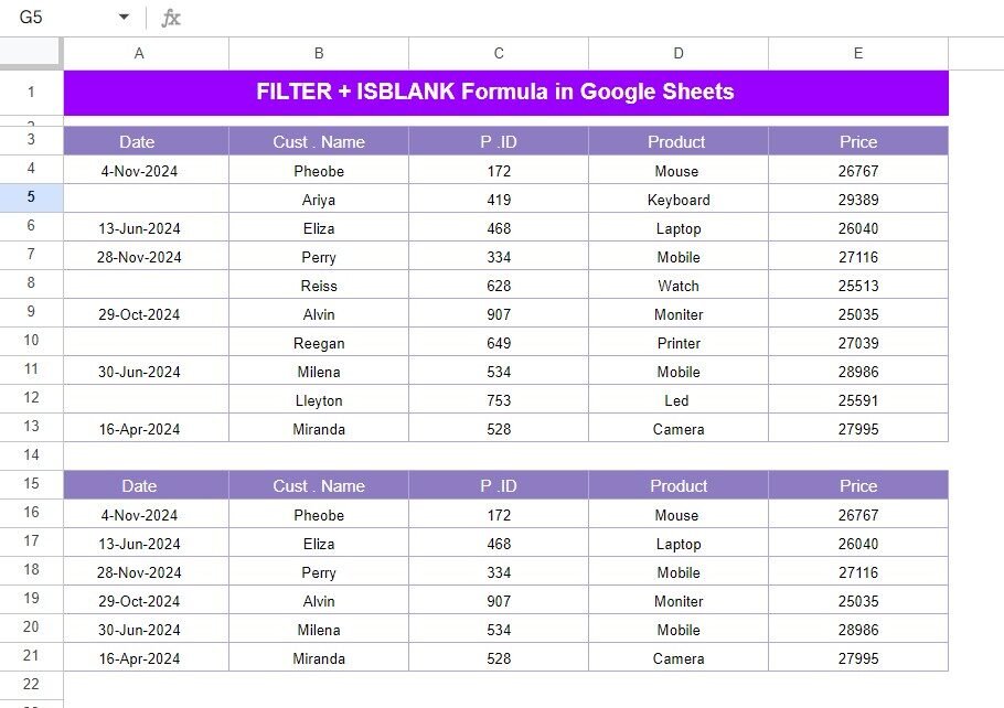
For our example, let’s consider we have a dataset located in the range A3 to E13 on Google Sheets. This set consists of columns like Date, Customer Name, Product ID, Product, and Price. Interestingly, some entries under the Date column are missing, and we need to exclude these to tidy up our data.

The Layout of Our Dataset
Here’s how our raw data looks:
The Formula That Does the Trick
Now, to focus only on rows with dates, we apply a nifty formula combining FILTER and ISBLANK:
=FILTER(A4:E13, NOT(ISBLANK(A4:A13)))

Let’s Break It Down
FILTER(A4
- This tells Google Sheets to consider the data in the specified range.
NOT(ISBLANK(A4
- This part works wonders by filtering out rows. ISBLANK checks if there are any empty date cells, and NOT ensures we skip these blanks.
Your New View
With our formula in action, the spreadsheet smartly omits any rows without date entries. Here’s the clear, filtered output you’ll see:
Why Does This Matter?
Using these functions not only saves precious time but also enables you to make quicker, more accurate decisions based on cleaner data. Perfect for anyone from marketers to data analysts or even casual spreadsheet users who want to up their data game.
Conclusion
And just like that, you’re on your way to becoming a Google Sheets guru! Dive into your spreadsheets with these handy functions and let them do the heavy lifting. You’ll be amazed at how simple and fun data handling can be. Go ahead, give it a try and watch your productivity soar!
Visit our YouTube channel to learn step-by-step video tutorials
Youtube.com/@NeotechNavigators
View this post on Instagram
Click here to Make the copy of this Template


