Do you want to filter your data based on specific criteria and find the minimum values in Google Sheets? You’re in the right place! In this post, we’ll explore how to use two powerful Google Sheets functions, FILTER and MINIFS Functions, together to streamline your data analysis.
In our example, we’ll walk through the process using a real-life dataset. We’ll explain everything in simple terms, so whether you’re a beginner or an experienced user, you’ll find this guide helpful and engaging!
Understanding the Dataset
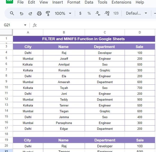
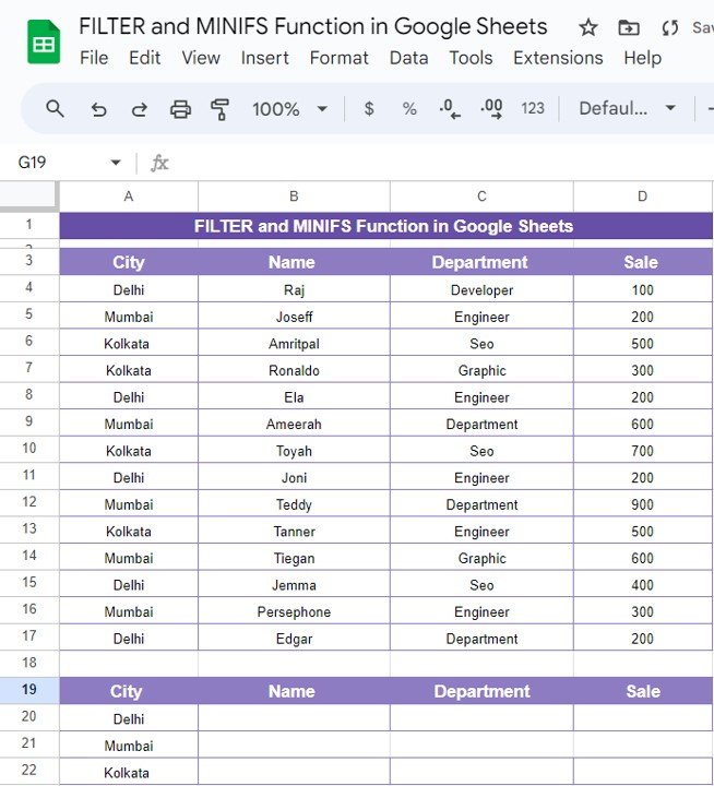
Before diving into the formulas, let’s take a look at the data we’ll be working with. Imagine we have a table with information on different employees, their cities, departments, and sales. Here’s how our data looks:
Our goal is to use the FILTER and MINIFS functions to pull out the rows that meet specific criteria and display only the ones with the minimum sales in each city. Ready to see how this works? Let’s dive in!
How the MINIFS Function Works
The MINIFS function is a handy tool when you need to find the smallest value in a dataset based on one or more criteria. In our case, we want to find the minimum sales amount for a specific city.
Here’s the formula we’ll use:
=MINIFS($D$3:$D$17, $A$3:$A$17, A20)
Let’s break this down:
$D$3:$D$17 refers to the range where our sales data is located.
$A$3:$A$17 refers to the city column where we’re applying our criteria.
A20 is the cell that contains the specific city we’re focusing on, such as “Delhi” or “Mumbai.”
This function will return the minimum sales figure for the chosen city, allowing us to easily identify the lowest performers.
Using the FILTER Function to Extract Data
Once we’ve identified the minimum sales figure with MINIFS, we can use the FILTER function to extract the relevant rows from the dataset. This is where the magic happens!
Here’s the FILTER formula we’ll be using:
=FILTER($B$3:$D$17, $D$3:$D$17 = MINIFS($D$3:$D$17, $A$3:$A$17, A20))
Now, let’s break this one down too:
$B$3:$D$17 is the range of data we want to return, which includes the name, department, and sales columns.
$D$3:$D$17 = MINIFS(…) ensures that only the rows where the sales values match the minimum sales for that city are returned.
By combining FILTER with MINIFS, we can narrow down our dataset to show only the rows with the lowest sales figures for a given city. Pretty cool, right?
The Output
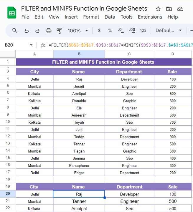
So, what do we get when we apply these formulas to our example dataset? Let’s take a look at the result:
As you can see, the FILTER function has successfully extracted the rows where the sales figures are the lowest for each city.
Why You Should Use FILTER and MINIFS in Google Sheets
Using FILTER and MINIFS together can make your data analysis process faster and more efficient. Here are some key benefits of using these functions:
- 🎯 Targeted Results: Easily focus on specific data points, like the lowest sales figures, without manually searching through your data.
- ⏱ Time-Saving: Once set up, these functions automatically update as your data changes, saving you from doing repetitive tasks.
- 📊 Better Insights: Quickly identify trends and patterns in your dataset by filtering out irrelevant data.
Conclusion
By mastering the FILTER and MINIFS functions, you’ll unlock a powerful combination that can transform how you work with data in Google Sheets. These formulas allow you to pull out the most relevant information, saving you time and improving your data analysis process.
Visit our YouTube channel to learn step-by-step video tutorials
Youtube.com/@NeotechNavigators
View this post on Instagram
Click here to Make the copy of this Template
