In this blog post, we’re diving into two of the most useful and efficient functions in Google Sheets: IFERROR and XLOOKUP Function. If you’ve ever worked with data, especially large sets of it, you’ve probably encountered errors or had trouble looking up specific information. Well, today, we’re going to tackle these common issues with the help of these two powerful functions. So, let’s get started with a clear example and some real-world applications!
By the end of this post, you’ll understand:
How to use the IFERROR function to manage errors in your data.
How to apply XLOOKUP to fetch specific data from a range.
How combining both functions makes your Google Sheets workflow smoother and error-free.
Let’s break this down step by step with an example.

The Scenario: What Are We Trying to Achieve?
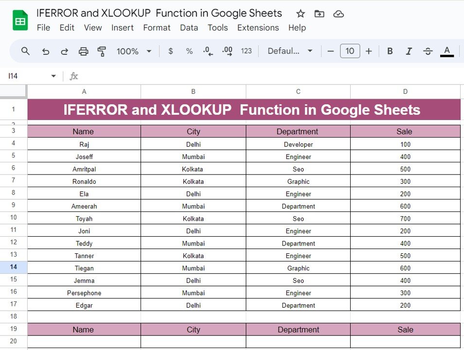
We have a dataset that includes the Name, City, Department, and Sales of employees. Our goal is to use the IFERROR and XLOOKUP functions to retrieve specific information about employees without encountering errors, especially if the data we’re searching for doesn’t exist.
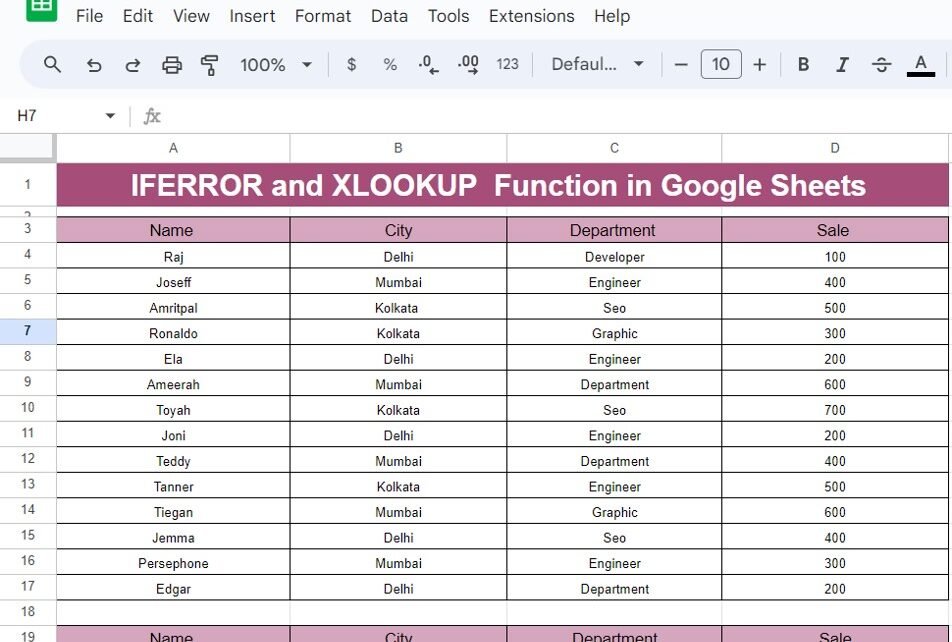
Here’s the data range we’re working with:
- The Problem: Fetching Data with Potential Errors
Suppose we want to look up the details of a person (like Ameerah) based on their name. If the name exists, we need to display their city, department, and sales. However, if the name doesn’t exist, we don’t want an ugly error showing up in our sheet. Instead, we want a blank cell or a custom message.
- The Solution: Using IFERROR and XLOOKUP Together
Here’s where the magic happens! By combining IFERROR and XLOOKUP, we can search for the name in the dataset and display the relevant details without any hassle.
The Formula:
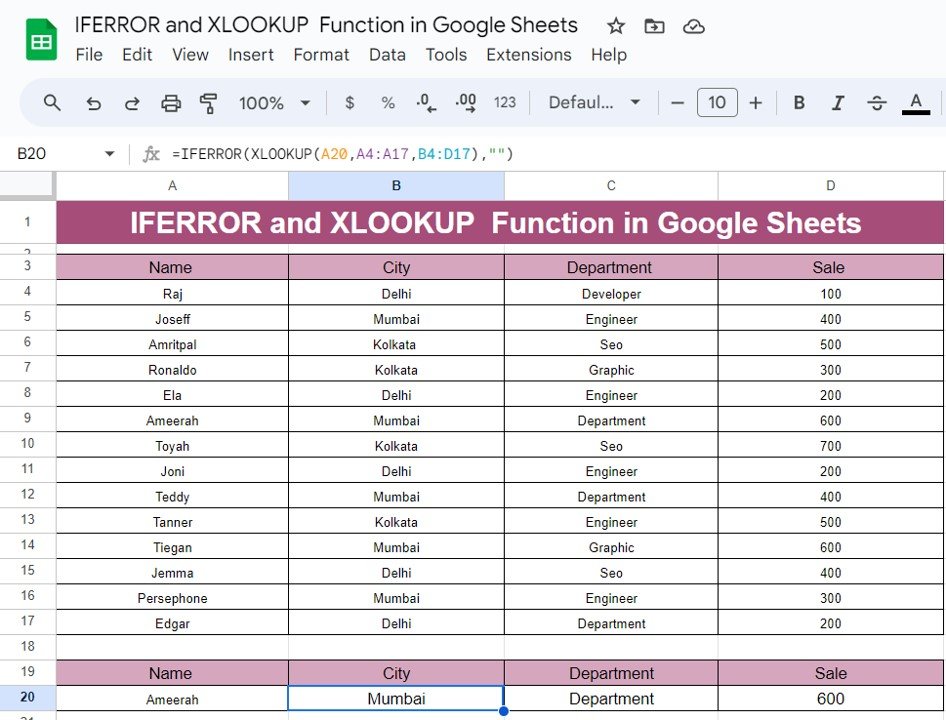
=IFERROR(XLOOKUP(A20,A4:A17,B4:D17),"")
Let’s break this down:
- XLOOKUP: This function looks for a value (in this case, the name in cell A20) within a range (A4) and returns data from the corresponding rows in columns B to D (the city, department, and sales).
- IFERROR: If XLOOKUP doesn’t find the value or encounters an error, this function catches the error and returns a blank value (or any custom message you prefer).
Explanation of the Formula:
- A20: This is the cell where the name we’re looking for is located.
- A4: This is the range where we are searching for the name.
- B4: These are the columns from which we want to return the data (City, Department, and Sales).
- “”: This tells the formula to return a blank cell if an error occurs, instead of displaying an error message.
Example Output
Let’s assume we’re searching for “Ameerah” in the dataset. When we apply the formula, we get the following result:
Perfect! The formula has successfully retrieved all the details for Ameerah from the dataset.
But what if we search for a name that doesn’t exist, like “John”? Instead of getting an error, our formula will simply return blank cells, keeping our sheet looking clean and professional.

Why Use IFERROR and XLOOKUP Function Together?
Using these functions in combination offers several advantages:
- Error-Free Data: You avoid annoying error messages like #N/A when data isn’t found.
- Professional Output: Blank cells or custom error messages look much cleaner than errors splashed across your sheet.
- Efficient Lookups: XLOOKUP allows for much more flexible and powerful lookups compared to the old VLOOKUP function.
Practical Application
Let’s consider a real-world scenario. Imagine you’re managing a sales team and need to pull up information about your employees. With the IFERROR and XLOOKUP functions, you can quickly and easily search for employees by name, see their department, and even their latest sales figures — all without worrying about errors cluttering your sheet.
Conclusion: Make Your Life Easier with IFERROR and XLOOKUP
These two functions are essential tools for anyone working with data in Google Sheets. Whether you’re trying to avoid errors or perform efficient lookups, IFERROR and XLOOKUP can significantly improve your workflow. Give them a try on your own dataset and see how much smoother your sheets become!
Visit our YouTube channel to learn step-by-step video tutorials
Youtube.com/@NeotechNavigators


