The VLOOKUP function in Google Sheets is a powerful tool that helps you find and return information from a large dataset. Whether you’re looking up sales data, customer information, or product details, the VLOOKUP function can save you loads of time by searching for specific values in your sheet.

In this blog post, we’ll walk you through how to use the VLOOKUP function in Google Sheets with a real-life example. By the end, you’ll feel confident using this function to streamline your data lookup tasks.

Table of Contents

What is the VLOOKUP Function?

The VLOOKUP function stands for “Vertical Lookup,” and it allows you to search for a specific value in one column of your Google Sheets and return a corresponding value from another column in the same row. It’s extremely useful for finding matching data quickly without manually sifting through your spreadsheet.

=VLOOKUP(search _key, range, index, [is _sorted])

search _key: The value you want to look up.
range: The table or range of cells where the lookup will happen.
index: The column number from where to retrieve the result (relative to the first column of the range).
is_sorted: Optional argument (FALSE for an exact match).
Real-Life Example: VLOOKUP to Find Sales Data

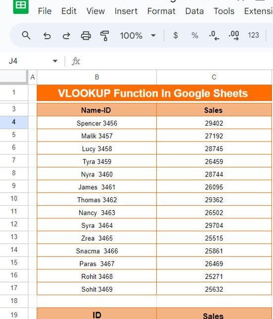
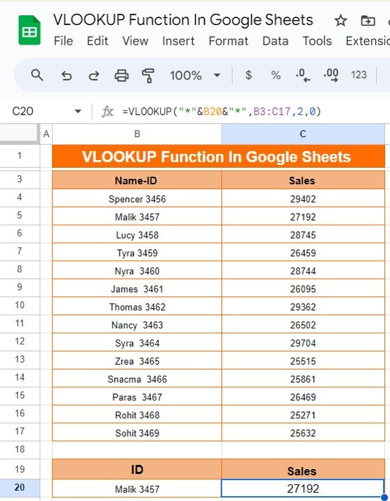
Let’s say we have a dataset with employee sales information. The dataset looks like this:

Now, let’s say you want to find the sales numbers for an employee using their Name-ID. Instead of manually searching, you can use the VLOOKUP function to quickly get the sales data.

How to Use the VLOOKUP Function

Set up your data:

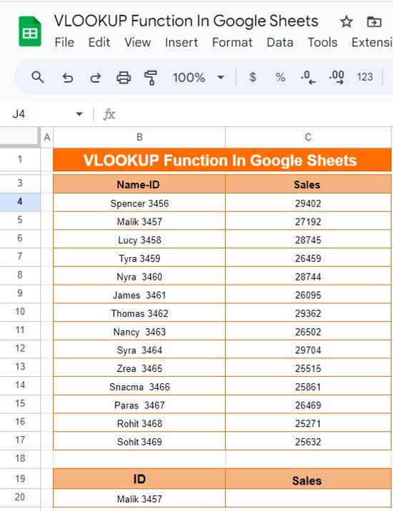
Make sure your data is properly structured in columns. In this case, we have Name-ID in column B and Sales in column C.

Use the VLOOKUP formula:

Let’s say you want to look up the sales figure for “Malik 3457.” You can use this formula in cell D20 to get the value:

=VLOOKUP("*"&B20&"*",B3:C17,2,0)

Breakdown of the formula:

“”&B20&””: This part of the formula uses wildcard characters (*) to search for any value that contains the Name-ID specified in cell B20.
B3: This is the range where we are looking for the value. Column B has the Name-ID and column C has the corresponding Sales.
2: This tells the formula to return the value from the second column in the specified range (which is the Sales column).
0: This ensures that the function looks for an exact match.

Output of the VLOOKUP Function

Once you’ve entered the formula, here’s what your output might look like:

The VLOOKUP function efficiently retrieves the sales data for “Malik 3457” without having to manually search through the dataset.

Advantages of Using VLOOKUP in Google Sheets

Quick Data Retrieval: With VLOOKUP, you can instantly find and return relevant information from large datasets.
Time-Saving: Instead of scrolling through rows of data, you can use the function to automatically search and pull the needed information.
Flexible Matching: Using wildcards, you can search for partial matches, making the function adaptable to many different use cases.

Final Thoughts

The VLOOKUP function is one of the most useful tools in Google Sheets for quickly finding data. Whether you’re looking up sales numbers, product prices, or employee details, the function simplifies the process and saves you time.

Visit our YouTube channel to learn step-by-step video tutorials

Youtube.com/@NeotechNavigators