VLOOKUP is the function most people learn first for pulling data from a table, but it can do much more than a single lookup. This guide covers 6 VLOOKUP tricks in Google Sheets: the standard lookup, VLOOKUP with COLUMN, VLOOKUP with MATCH, a double (nested) VLOOKUP, error handling with IFERROR, and ageing buckets with an approximate match.
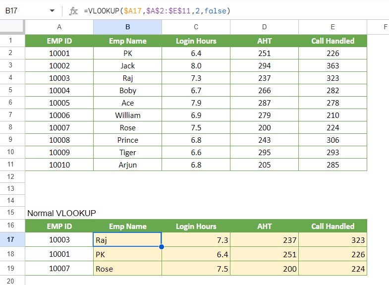
Every example uses the same small call-centre dataset from the free practice file: ten employees with EMP ID, Emp Name, Login Hours, AHT and Call Handled. The results quoted here match the practice file data shown in the screenshots, so you can check your own formulas against them.
🎥 Watch the Video Tutorial
Make a Copy of the Free Practice File
VLOOKUP Syntax in Google Sheets
=VLOOKUP(search_key, range, index, [is_sorted])| Argument | Meaning | In the examples |
|---|---|---|
| search_key | The value to find. It must be in the first column of the range. | An EMP ID such as 10003 |
| range | The table to search. | $A$2:$E$11 (or $A$1:$E$11 with headers) |
| index | Which column of the range to return; 1 is the first column. | 2 = Emp Name, 3 = Login Hours, 4 = AHT, 5 = Call Handled |
| is_sorted | FALSE (or 0) for an exact match; TRUE (or 1, or omitted) for an approximate match on sorted data. | FALSE for IDs, TRUE for age buckets |
The data table runs from A1:E11. The IDs go from 10001 (PK) to 10010 (Arjun). A second table in I1:J11 maps each Login ID (20001–20010) to an EMP ID (10001–10010).
Trick 1: Normal VLOOKUP
To return the employee name for the ID in A17, use this formula:
=VLOOKUP($A17,$A$2:$E$11,2,FALSE)For ID 10003 it returns Raj. Change the index to 3, 4 and 5 to get Login Hours 7.3, AHT 237 and Call Handled 323. The $ before A keeps the lookup column fixed when you copy the formula across, and the locked range stays put when you copy down.
Trick 2: VLOOKUP with COLUMN() for Copy-Across Formulas
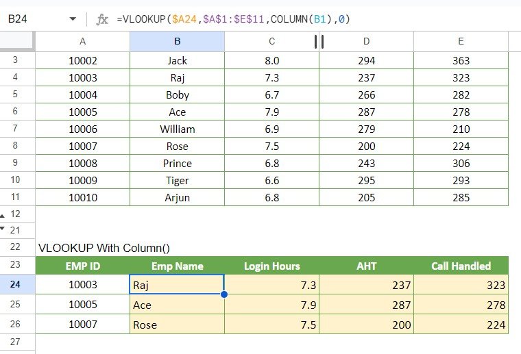
Typing 2, 3, 4 and 5 by hand is slow and easy to get wrong. COLUMN() returns the column number of a reference, so it can supply the index for you:
=VLOOKUP($A24,$A$1:$E$11,COLUMN(B1),0)COLUMN(B1) = 2, so B24 returns the name. When you copy the formula to the right, it becomes COLUMN(C1) = 3, COLUMN(D1) = 4 and so on. For ID 10005 the row fills with Ace, 7.9, 287, 278. This works because the output table has its columns in the same order as the source table.
For a deeper look, see our guide to VLOOKUP with the COLUMN function.
Trick 3: VLOOKUP with MATCH for Column Order That Changes
If your output headers are in a different order from the source, or someone may insert columns later, let MATCH find the column by its header name. This version is not shown in the screenshots, but you can drop it into the same output table used for Trick 2:
=VLOOKUP($A24,$A$1:$E$11,MATCH(B$23,$A$1:$E$1,0),0)MATCH looks up the header in B23 (“Emp Name”) inside the source header row A1:E1 and returns its position, 2. For a column headed “Login Hours”, MATCH returns 3, so ID 10003 gives 7.3. The mixed reference B$23 keeps the header row fixed while the column moves. A full walkthrough is in VLOOKUP with MATCH in Google Sheets.
Trick 4: Double VLOOKUP (Lookup Through a Mapping Table)
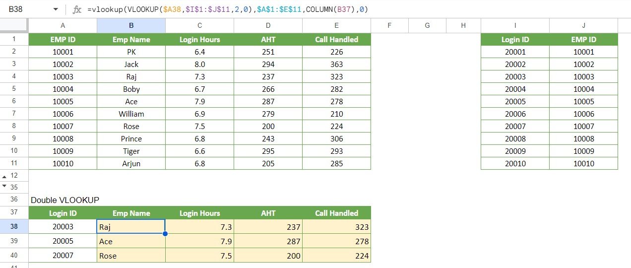
Sometimes you only have a Login ID, but the data is keyed by EMP ID. A nested VLOOKUP first converts one ID to the other, then fetches the data:
=VLOOKUP(VLOOKUP($A38,$I$1:$J$11,2,0),$A$1:$E$11,COLUMN(B37),0)- The inner VLOOKUP finds Login ID 20003 in I1:J11 and returns EMP ID 10003.
- The outer VLOOKUP uses 10003 to return Raj, and copied across, 7.3, 237, 323.
In the practice file, 20005 returns Ace and 20007 returns Rose.
Trick 5: Error Handling with IFERROR
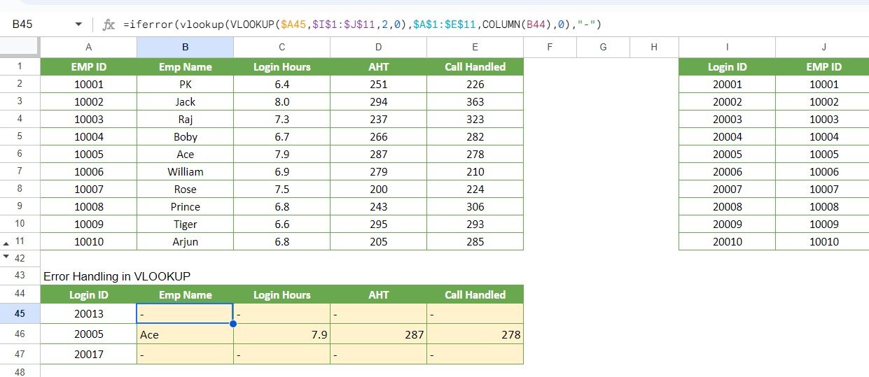
If a Login ID does not exist, VLOOKUP returns #N/A, which looks broken in a report. Wrap the formula in IFERROR to show something cleaner:
=IFERROR(VLOOKUP(VLOOKUP($A45,$I$1:$J$11,2,0),$A$1:$E$11,COLUMN(B44),0),"-")Login IDs 20013 and 20017 are not in the mapping table, so their rows show “-“. Login ID 20005 still returns Ace, 7.9, 287, 278. You can replace “-” with “Not found” or an empty string “”.
Trick 6: Ageing Buckets with Approximate Match
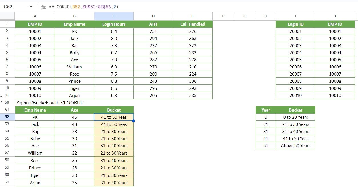
With is_sorted set to TRUE (or left out), VLOOKUP returns the row for the largest value that is less than or equal to the search key. That makes it ideal for grouping numbers into bands. The bucket table has its headers (Year, Bucket) in H51:I51 and lists the lower bound of each band in H52:I56:
| Year (lower bound) | Bucket |
|---|---|
| 0 | 0 to 20 Years |
| 21 | 21 to 30 Years |
| 31 | 31 to 40 Years |
| 41 | 41 to 50 Years |
| 51 | Above 50 Years |
=VLOOKUP(B52,$H$52:$I$56,2)PK, aged 46, lands in 41 to 50 Years, because 41 is the largest lower bound not above 46. Raj (23) gets 21 to 30 Years and Ace (31) gets 31 to 40 Years. The first column of the bucket table must be sorted in ascending order.
The same pattern works for invoice ageing (0–30, 31–60, 61–90 days), commission slabs and grade bands.
Common VLOOKUP Errors and Fixes
| Error | Cause | Fix |
|---|---|---|
| #N/A | The key is not in the first column, or numbers are stored as text in one table | Check the spelling and the data type; convert with VALUE() or TO_TEXT(). |
| #REF! | The index is larger than the number of columns in the range | Widen the range or lower the index. |
| Wrong value returned | is_sorted left blank on an exact-match lookup | Add FALSE or 0 as the fourth argument. |
| Results shift when copied | Range not locked with $ | Use $A$2:$E$11. |
| Can’t look to the left | VLOOKUP only returns columns to the right of the key | Use XLOOKUP or INDEX/MATCH. |
Tips for Using These VLOOKUP Tricks in Google Sheets
- Keep IDs unique. VLOOKUP returns the first match only.
- Use COLUMN or MATCH instead of typed index numbers in any table you copy across.
- Wrap reports in IFERROR, but only after the formula is tested, so it does not hide real mistakes.
- For new sheets, consider XLOOKUP. It can look left and has a built-in “if not found” argument.
Keep learning with our complete VLOOKUP guide for Google Sheets, the VLOOKUP real-life example and IFERROR with XLOOKUP.
If you want to go further with structured lessons on lookups and other functions, the Excel AI Mastery: 100 Formulas course on NextGenTemplates Academy covers VLOOKUP, XLOOKUP and INDEX/MATCH with practice files. The syntax is the same in Excel and Google Sheets.
Frequently Asked Questions
Can VLOOKUP search from right to left?
No. VLOOKUP always searches the first column of the range and returns a column to its right. To look left, use XLOOKUP or INDEX with MATCH.
What does FALSE or 0 mean at the end of VLOOKUP?
It forces an exact match. Without it, Google Sheets assumes sorted data and may return the closest smaller value instead of the one you want.
How do I return several columns with one VLOOKUP?
Copy a VLOOKUP that uses COLUMN() as the index across the row. In Google Sheets you can also pass an array of indexes, for example =ARRAYFORMULA(VLOOKUP(A17,$A$2:$E$11,{2,3,4,5},FALSE)).
Why does VLOOKUP return #N/A when the value is clearly there?
Usually one value is a number and the other is text (for example “10003” typed with an apostrophe), or there are extra spaces. Use TRIM and check the format of both cells.
When should I use approximate match?
Use it for ranges and bands, such as ageing buckets, tax slabs or grades, where the first column lists sorted lower bounds.
Wrapping Up
These six tricks cover most real lookup tasks: a plain lookup, copy-across formulas with COLUMN, header-driven lookups with MATCH, mapping through a second table, clean error handling and grouping into buckets. Make a copy of the practice file, change a few IDs, and rebuild each formula yourself. That is the quickest way to make them second nature.
Copy the Free VLOOKUP Practice File
📅 Last updated: October 2026