The RANK function in Google Sheets tells you the position of a number within a list: 1 for the highest, 2 for the next, and so on (or the other way round if you choose ascending order). It is the quickest way to turn a column of scores, sales or times into a league table without sorting the data.
This guide is for teachers, team leads and analysts who need a clean ranking that updates by itself. You will work through a real example of 12 students and their marks, see exactly how ties are handled, and learn variations for ascending ranks, average ranks for ties, unique ranks and a top-3 list.
RANK Syntax and Arguments
=RANK(value, data, [is_ascending])| Argument | What it means | In the example |
|---|---|---|
| value | The number you want to rank. | B4 (Nyra’s 75%) |
| data | The full list of numbers to rank against. Lock it with dollar signs so it does not move when you copy the formula. | $B$4:$B$15 |
| is_ascending | Optional. 0 or FALSE (the default) ranks the highest value as 1. 1 or TRUE ranks the lowest value as 1. | 0 |
Google Sheets also has RANK.EQ, which behaves the same as RANK, and RANK.AVG, which handles ties differently (see the variations below).
The Example Data
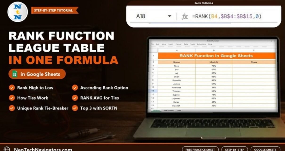
The practice sheet lists 12 students in column A (Name) with their marks in column B (Mark%), rows 4 to 15. Column C, Rank, is empty to start with.

Step-by-Step: Rank the Students
- Click the Rank cell for the first student (Nyra, row 4).
- Enter the formula below and press Enter.
- Fill it down to row 15 by dragging the fill handle or double-clicking it.
=RANK(B4,$B$4:$B$15,0)- B4 is relative, so it becomes B5, B6 and so on as you fill down.
- $B$4:$B$15 is absolute, so every row is compared against the same 12 marks.
- 0 means descending: the highest mark gets rank 1.
The Result
In the practice file the ranks are placed in a separate block (A17:A29) under a Rank heading, with the formula in A18 pointing at B4. The results line up with the students in the same order:

| Name | Mark% | Rank |
|---|---|---|
| Nyra | 75% | 5 |
| tyra | 67% | 6 |
| raj | 87% | 2 |
| Vivan | 98% | 1 |
| Sourabh | 45% | 10 |
| James | 67% | 6 |
| Homense | 34% | 12 |
| Thomas | 56% | 8 |
| Sypyra | 78% | 4 |
| Unjames | 85% | 3 |
| Kyrav | 48% | 9 |
| Siyansh | 39% | 11 |
Vivan’s 98% is the highest, so he ranks 1; Homense’s 34% is the lowest, so he ranks 12.
How ties work
tyra and James both scored 67%, so both receive rank 6. RANK then skips rank 7, and the next student, Thomas with 56%, gets rank 8. This is called “competition ranking” and it is the standard behaviour of RANK and RANK.EQ.
Practical Variations
1. Ascending rank (lowest = 1)
Use 1 as the third argument when a smaller number is better, such as race times, costs or defects. With the practice data, Homense becomes rank 1 and Nyra rank 8:
=RANK(B4,$B$4:$B$15,1)2. Average rank for ties with RANK.AVG
RANK.AVG gives tied values the average of the positions they occupy. tyra and James share positions 6 and 7, so both get 6.5:
=RANK.AVG(B4,$B$4:$B$15,0)3. Unique rank with a tie-breaker
When every row needs a different number (for example, to look up “rank 7” later), add a running count of earlier duplicates. tyra stays 6 and James becomes 7:
=RANK(B4,$B$4:$B$15,0)+COUNTIF($B$4:B4,B4)-1The expanding range $B$4:B4 counts how many times the value has appeared so far, so the first occurrence gets the base rank and later ones move down by one.
4. List the top 3 students
SORTN returns the top rows directly, without a helper column. This returns Vivan 98%, raj 87% and Unjames 85%:
=SORTN(A4:B15,3,0,2,FALSE)5. Label the top performers
Combine RANK with IF to show a label next to the leaders (here C4 holds the rank):
=IF(C4<=3,"Top 3","")RANK vs RANK.EQ vs RANK.AVG vs PERCENTRANK
| Function | Ties | Output |
|---|---|---|
| RANK | Same rank, next rank skipped | Whole number position |
| RANK.EQ | Same as RANK | Whole number position |
| RANK.AVG | Average of the tied positions | Can be a decimal (6.5) |
| PERCENTRANK | Shared percentile | A value from 0 to 1 showing relative standing |
Common Errors and Fixes
- Ranks change or repeat strangely after filling down: the data range was not locked. Use
$B$4:$B$15, notB4:B15. - #N/A: the value is not found in the data range, usually because the range stops one row short or the value cell points outside it.
- A row is skipped or ranked oddly: the mark is stored as text (for example “75 %” with a space). Re-enter it as a number and use Format > Number > Percent.
- Ranks are upside down: the third argument is 1 when you wanted 0, or the other way round.
- Two people share a rank and you need unique numbers: use the COUNTIF tie-breaker shown above.
Tips
- Rank the underlying numbers, not a rounded display. Two marks that both show as 67% may differ in the decimals, which affects the result.
- If the list grows, use an open range such as
$B$4:$B; RANK ignores blank cells. - Add conditional formatting on the Rank column (Format > Conditional formatting, “Less than or equal to” 3) to highlight the leaders.
For a longer walkthrough with more scenarios, see the comprehensive guide to the RANK function. For percentile standing instead of position, read how to use PERCENTRANK. To pull the top or bottom rows into a separate table, try SORT and FILTER with an example or FILTER and LARGE in Google Sheets, and for turning marks into letters, assign grades with the IF function.
If you would like guided practice with ranking, lookup and statistical formulas, the Excel AI Mastery: 100 Formulas course on NextGenTemplates Academy covers them lesson by lesson, and the same functions work in Google Sheets.
Frequently Asked Questions
How do I rank from highest to lowest in Google Sheets?
Use =RANK(B4,$B$4:$B$15,0) or leave out the last argument. The highest value gets rank 1.
Why do two values have the same rank?
They are equal. RANK gives tied values the same position and skips the next number, which is why tyra and James both show 6 and Thomas shows 8.
How can I give every row a unique rank?
Add a tie-breaker: =RANK(B4,$B$4:$B$15,0)+COUNTIF($B$4:B4,B4)-1. Earlier duplicates keep the base rank and later ones move down by one.
What is the difference between RANK and RANK.AVG?
RANK gives tied values the same whole-number rank. RANK.AVG gives them the average of the positions they cover, such as 6.5 for two values sharing positions 6 and 7.
Does RANK update when the marks change?
Yes. RANK recalculates immediately whenever a value in the data range changes, so the league table always reflects the current numbers.
Wrapping Up
With one formula, =RANK(B4,$B$4:$B$15,0), the 12 students were ranked from Vivan at 1 to Homense at 12, with the 67% tie shared at rank 6. Switch the last argument for ascending order, use RANK.AVG or a COUNTIF tie-breaker when ties matter, and SORTN when you only need the top few. Copy the practice sheet with File > Make a copy and try it on your own scores.
📅 Last updated: October 2026