The DMIN function in Google Sheets returns the smallest value in one column of a table, but only for the rows that match the conditions you set in a separate criteria block. Think of it as MIN with a built-in filter: you describe which rows count, and DMIN finds the lowest number among them.
This guide is for anyone who keeps sales, stock or order data in a table with headers and wants answers like “what is the lowest sale for this seller and product?” without sorting or filtering by hand. You will see the syntax, a worked example with real numbers from the practice sheet, five variations, and the mistakes that most often break a DMIN formula.
DMIN Syntax and Arguments
=DMIN(database, field, criteria)| Argument | What it means | In the example |
|---|---|---|
| database | The full table, including the header row. DMIN uses the headers to find columns. | A3:D15 |
| field | The column to take the minimum from. Use the header text in quotes, a cell that contains the header, or the column number within the table. | C17 (a cell holding “Total Price”) |
| criteria | A small block with header names on the first row and the conditions underneath. Conditions on the same row are joined with AND; separate rows are joined with OR. | A17:B18 |
DMIN belongs to the database function family with DGET, DMAX, DSUM, DAVERAGE and DCOUNT. They all share this same three-argument pattern.
The Example Data
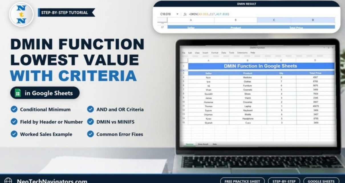
The practice sheet has a 12-row sales table in A3:D15 with four headers: Seller, Product, Qty and Total Price.

| Seller | Product | Qty | Total Price |
|---|---|---|---|
| Nyra | Medicine | 8 | 4567 |
| tyra | Clothes | 7 | 8765 |
| raj | Furniture | 6 | 9876 |
| Vivan | Cosmetic | 5 | 3456 |
| Sourabh | Shoes | 4 | 7654 |
| James | Watch | 3 | 2345 |
| Homense | Crocaries | 2 | 8907 |
| Thomas | Laptop | 1 | 45678 |
| Sypyra | Keyboard | 9 | 3456 |
| Unjames | Mobile | 6 | 3457 |
| Kyrav | Headphone | 5 | 8765 |
| Siyansh | C.p.u | 3 | 3456 |
Worked Example: Lowest Total Price for a Seller and Product
Below the table, the practice sheet has a criteria block in A17:B18: the headers Seller and Product on row 17, and the values tyra and Clothes on row 18. Cell C17 holds the header Total Price, and the result goes in C18:
=DMIN(A3:D15,C17,A17:B18)
How Google Sheets works it out:
- It reads the criteria headers (Seller, Product) and finds those columns in A3:D15.
- It keeps only rows where Seller is tyra and Product is Clothes. Because both conditions are on the same row of the criteria block, both must be true.
- It looks at the Total Price column for those rows and returns the smallest value.
Only one row matches (tyra, Clothes, 7, 8765), so the result is 8765. With more matching rows, DMIN would return the lowest of them.
Five Practical Variations
Each variation uses the same table. Only the criteria block (or the field) changes.
1. Use a comparison in the criteria
Put Qty in a criteria header cell and >5 below it. Five rows have a quantity above 5 (Nyra, tyra, raj, Sypyra and Unjames), and the lowest Total Price among them is Sypyra’s:
=DMIN(A3:D15,"Total Price",F3:F4)Result: 3456. Here F3 holds Qty and F4 holds >5.
2. OR logic with two criteria rows
To find the cheaper of Laptop or Watch, put Product in the header and Laptop and Watch on two separate rows underneath (for example H3:H5):
=DMIN(A3:D15,"Total Price",H3:H5)Result: 2345 (James, Watch). Rows in the criteria block are alternatives, so either product counts.
3. Filter on the same column you measure
Criteria can test the Total Price column itself. With Total Price as the header and >5000 below, DMIN returns the smallest sale above 5000:
=DMIN(A3:D15,"Total Price",J3:J4)Result: 7654 (Sourabh, Shoes).
4. Pick the field by number
The field can be the column position inside the database. Qty is the third column, so this returns the lowest quantity for the tyra and Clothes criteria:
=DMIN(A3:D15,3,A17:B18)Result: 7. Using the header text is safer, because a column number breaks silently if someone inserts a column.
5. The same answer with MINIFS
If you prefer conditions inside the formula instead of a criteria block, MINIFS gives the same answer:
=MINIFS(D4:D15,A4:A15,"tyra",B4:B15,"Clothes")Result: 8765. DMIN is handy when users should change conditions in visible cells; MINIFS is more compact for fixed rules. For the overall lowest price with no conditions, plain =MIN(D4:D15) returns 2345.
DMIN vs MIN vs MINIFS
| Function | Conditions | Best for |
|---|---|---|
| MIN | None | The lowest value in a range |
| MINIFS | Written inside the formula, all joined with AND | Fixed conditions, quick one-off checks |
| DMIN | Kept in a criteria block on the sheet; supports AND and OR | Reports where people change the filter in cells, and OR conditions without extra formulas |
Common Errors and Fixes
- #VALUE! or an unexpected error: the field text does not match a header exactly. “Total price” with a different spelling or an extra space will not be found. Point the field at the header cell instead of typing it.
- The database range has no header row: DMIN needs the headers. Start the range on the header row (A3, not A4).
- Criteria headers do not match: the headers in the criteria block must be the same as the table headers. Copy and paste them rather than retyping.
- The result is the overall minimum: the criteria range includes an empty row. A blank criteria row matches every record, so check that the range stops at the last filled row.
- The result is 0: no row met the conditions, so check spelling in the criteria cells. A zero here usually means “nothing matched” rather than a real minimum of zero.
Tips
- Place the criteria block above or beside the table, with a clear label, so other users can see and change it.
- Use a dropdown (Insert > Dropdown) in the criteria cells so people can only pick valid sellers or products.
- Keep the database range a little larger than the data, or use whole columns like
A3:D, so new rows are included. - Reuse the same criteria block with DMAX, DSUM or DAVERAGE to build a small summary panel from one set of conditions.
For a second example with a different dataset, read DMIN in Google Sheets with conditional filtering. The sister functions are covered in how to use the DMAX function and the DGET function with a practical example, and the formula-based alternative in the MINIFS function in Google Sheets.
If you want structured practice with conditional formulas like these, the Excel AI Mastery: 100 Formulas course on NextGenTemplates Academy walks through database and lookup functions with exercises; the same logic applies in Google Sheets.
Frequently Asked Questions
What is the difference between DMIN and MINIFS in Google Sheets?
Both return a conditional minimum. MINIFS takes its conditions as formula arguments, while DMIN reads them from a criteria block on the sheet, which also lets you use OR logic by adding rows.
Can DMIN use more than one condition?
Yes. Put several headers side by side in the criteria block for AND conditions, as in the tyra and Clothes example, or stack values on separate rows for OR conditions.
Can the field argument be a number?
Yes. A number refers to the column position inside the database range, so 4 means the fourth column (Total Price in the example). Header text is easier to read and safer when columns move.
Does DMIN accept wildcards or comparison operators?
Comparison operators such as >5, <=100 or <>Clothes work in the criteria cells. Test any wildcard pattern on your own data before relying on it in a report.
Why does DMIN return the lowest value of the whole table?
The criteria range almost always contains an empty row. An empty criteria row matches everything, so shrink the range to the filled rows only.
Wrapping Up
DMIN finds the smallest value for exactly the rows you describe. In the example, =DMIN(A3:D15,C17,A17:B18) returned 8765 for tyra’s Clothes sale, and small changes to the criteria block answered other questions: 3456 for quantities above 5, 2345 for Laptop or Watch, and 7654 for sales above 5000. Make a copy of the practice sheet with File > Make a copy and try your own criteria.
📅 Last updated: October 2026