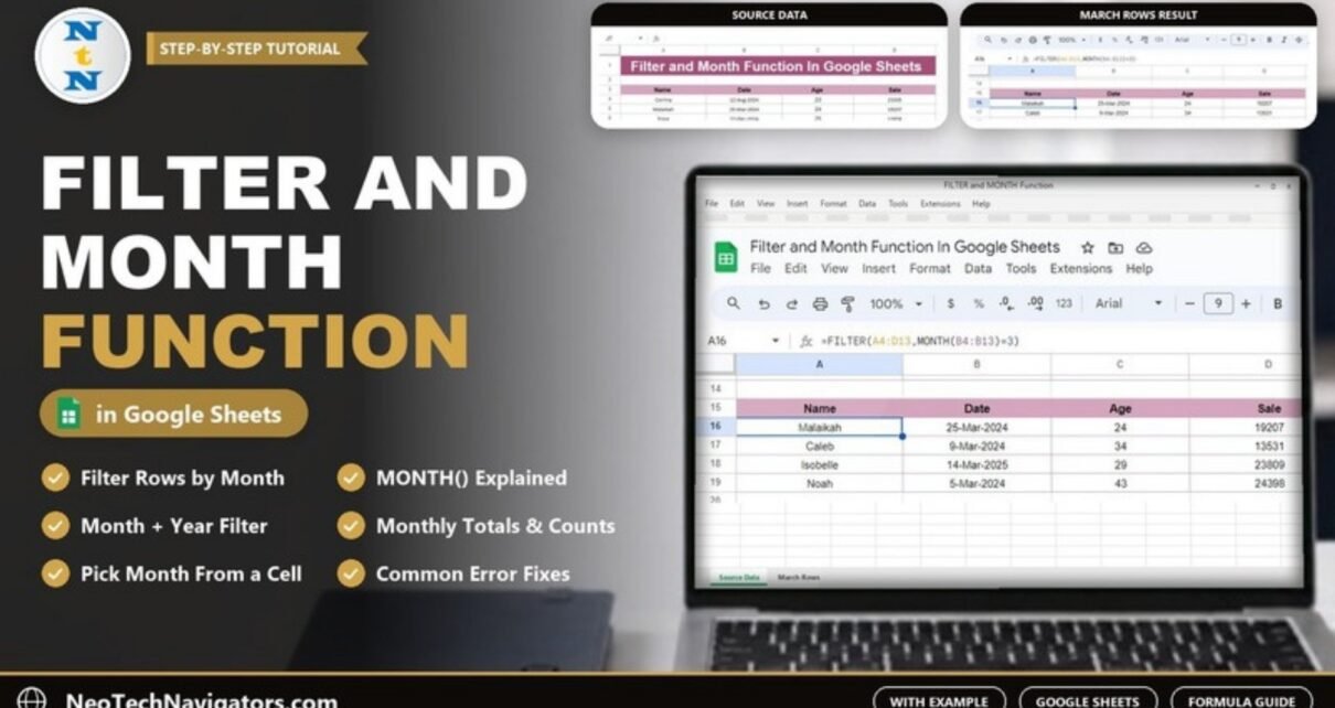
The FILTER and MONTH function in Google Sheets let you pull out every row that falls in a particular month with one formula. MONTH turns each date into a number from 1 to 12, and FILTER keeps only the rows where that number matches the month you want. The result is a live list that updates whenever the data changes.
In this example we take a ten-row list of Name, Date, Age and Sale and return only the March entries, whatever the year. You will see the syntax, how the formula works, the exact result, five variations (month plus year, a month picked from a cell, totals and more) and the errors to watch for. It is useful for anyone who reports sales, bookings or expenses by month.
The Sample Data
The data sits in A3:D13: headers in row 3 and ten records in rows 4 to 13. The dates run from 5-Mar-2024 to 14-Mar-2025, and four of them fall in March.

FILTER and MONTH Syntax
| Function / argument | What it means |
|---|---|
FILTER(range, condition1, [condition2, …]) |
Returns the rows of range where every condition is TRUE. |
range |
The data to return, here A4:D13. |
condition1 |
A TRUE/FALSE test with the same number of rows as range. |
MONTH(date) |
Returns the month of a date as a number: 1 for January through 12 for December. |
The Formula: Show Only March Rows
Copy the headers into row 15, click A16 and enter:
=FILTER(A4:D13, MONTH(B4:B13)=3)How it works
MONTH(B4:B13)converts each date in the Date column to a month number. 25-Mar-2024 becomes 3, 12-Aug-2024 becomes 8, and so on.=3compares each of those numbers with 3 and produces TRUE for March and FALSE for everything else.FILTER(A4:D13, …)returns the full rows that are TRUE and spills them below A16.
The Result
Four rows come back: Malaikah (25-Mar-2024, age 24, sale 19207), Caleb (9-Mar-2024, 34, 13531), Isobelle (14-Mar-2025, 29, 23809) and Noah (5-Mar-2024, 43, 24398). Note that Isobelle’s row is from 2025. MONTH only looks at the month, so March of any year is included.

5 Practical Variations
1. Limit the result to one month of one year
Add a YEAR condition. FILTER treats each extra condition as AND:
=FILTER(A4:D13, MONTH(B4:B13)=3, YEAR(B4:B13)=2024)Isobelle’s 2025 row drops out, leaving Malaikah, Caleb and Noah.
2. Pick the month from a cell
Type a month number in F2 and reference it, so anyone can switch the month without editing the formula:
=FILTER(A4:D13, MONTH(B4:B13)=F2)With 8 in F2 the result is Corrina (12-Aug-2024) and Leighton (26-Aug-2024). With 12 it is Trixie and Cohan. To make F2 friendlier, add a drop-down of 1 to 12 with Insert > Drop-down.
3. Total the sales for a month
Wrap the Sale column in SUM:
=SUM(FILTER(D4:D13, MONTH(B4:B13)=3))19207 + 13531 + 23809 + 24398 = 80945.
4. Count the rows for a month
COUNTIF cannot apply MONTH to a range, but SUMPRODUCT can:
=SUMPRODUCT(--(MONTH(B4:B13)=3))This returns 4.
5. Return a whole quarter
Use a range of months. For January to March:
=FILTER(A4:D13, MONTH(B4:B13)<=3)The sample has no January or February dates, so the same four March rows appear. To sort the output by date, wrap it in SORT as shown in our guide to SORT and FILTER functions.
Common Errors and Fixes
| Problem | Why it happens | Fix |
|---|---|---|
| #N/A – No matches are found in FILTER evaluation | No date falls in that month (for example January in this data). | Wrap it: =IFERROR(FILTER(…), "No entries this month"). |
| #VALUE! from MONTH | A date was typed as text that Google Sheets cannot recognise as a date, such as “5th of March”, so MONTH cannot read it. | Convert the column with Format > Number > Date or re-enter the dates. |
| Blank rows appear in a December filter | An empty cell is treated as day zero (30-Dec-1899), so MONTH returns 12. | Add a check: =FILTER(A4:D13, MONTH(B4:B13)=12, B4:B13<>""). |
| #REF! – array result was not expanded | Cells in the spill area already contain data. | Clear the cells below and to the right of the formula. |
Where Filtering by Month Is Useful
Most business data is logged by date, but most reports are read by month. A FILTER and MONTH formula bridges that gap without pivot tables or manual copying. Some everyday examples:
- Monthly sales review: list every sale in the month under review and total it with the SUM version above.
- Birthday or anniversary lists: because MONTH ignores the year, a single formula lists everyone with a birthday in a given month, whatever year they were born.
- Expense claims: pull one month’s receipts from a running log before submitting a claim.
- Subscription renewals: show the customers whose renewal date falls next month so you can contact them early.
- Seasonal comparisons: leave out the YEAR condition to compare every March on record side by side.
Put the month number in a cell and the formula on its own tab, and you have a simple monthly report page that anyone in the team can use by changing one value.
Tips for Filtering by Month
- Use open-ended ranges such as
A4:DandB4:Bif new rows are added regularly, and include theB4:B<>""check from the table above. - To show month names next to the results, use TEXT:
=TEXT(B4,"mmmm")returns “March”. Our TEXT and MONTH function guide covers this in detail. - For a date range that crosses month boundaries, compare dates directly:
B4:B13>=DATE(2024,3,1)andB4:B13<=EOMONTH(DATE(2024,3,1),0). See the EOMONTH guide for more. - The same FILTER pattern works with other tests, for example removing undated rows with FILTER and ISBLANK.
If you would like to build these skills in order, the 100 formulas course on NextGenTemplates Academy covers date, lookup and filtering functions with practice exercises.
Frequently Asked Questions
Why does my March filter include dates from another year?
MONTH returns only the month number, so 14-Mar-2025 and 5-Mar-2024 both give 3. Add YEAR(B4:B13)=2024 as a second condition to limit it to one year.
Can I filter by month name instead of number?
Yes. Compare the TEXT of each date: =FILTER(A4:D13, TEXT(B4:B13,"mmm")="Mar"). Numbers are simpler and avoid spelling issues, though.
How do I filter for the current month automatically?
Compare with today’s date: =FILTER(A4:D13, MONTH(B4:B13)=MONTH(TODAY()), YEAR(B4:B13)=YEAR(TODAY())). The result changes on the first day of each month.
Does the result update when I add new rows?
Only if the new rows fall inside the ranges in the formula. Use open-ended ranges like A4:D to include future rows.
Can I show the month result on a different tab?
Yes. Put the formula on a new tab and add the sheet name to each range, for example =FILTER(Data!A4:D13, MONTH(Data!B4:B13)=3). This keeps the original data untouched and gives you a clean report page that you can share or print on its own.
Does this work in Excel?
Yes. Excel 365 and Excel 2021 support =FILTER(A4:D13, MONTH(B4:B13)=3). For several conditions in Excel, multiply them inside one argument: (MONTH(B4:B13)=3)*(YEAR(B4:B13)=2024).
Wrapping Up
=FILTER(A4:D13, MONTH(B4:B13)=3) pulled the four March records out of the list in one step, and small changes turn it into a month picker, a monthly total or a single-year view. Recreate the ten-row table above, try each variation, then point the formula at your own sales or expense log.
📅 Last updated: October 2026