Your manager sends three quick questions. How much did each region sell? Who closed the most orders? And how is every month trending? In front of you there are sixty rows of raw sales data. You could add it up with a calculator, or you can let Google Sheets answer every question in a few seconds.
In this step-by-step tutorial you will learn five ways to summarize data in Google Sheets (SUMIFS, COUNTIFS, SPARKLINE, a pivot table and QUERY) plus a bonus trick that needs no formula at all. Every screenshot below comes from the finished practice file, so you can check your result at each step.
Free practice file: make your own copy of the practice sheet and type along. The download at the end of this post has the view link, the copy link and the full formula cheat sheet.
Watch the video tutorial
Video overview
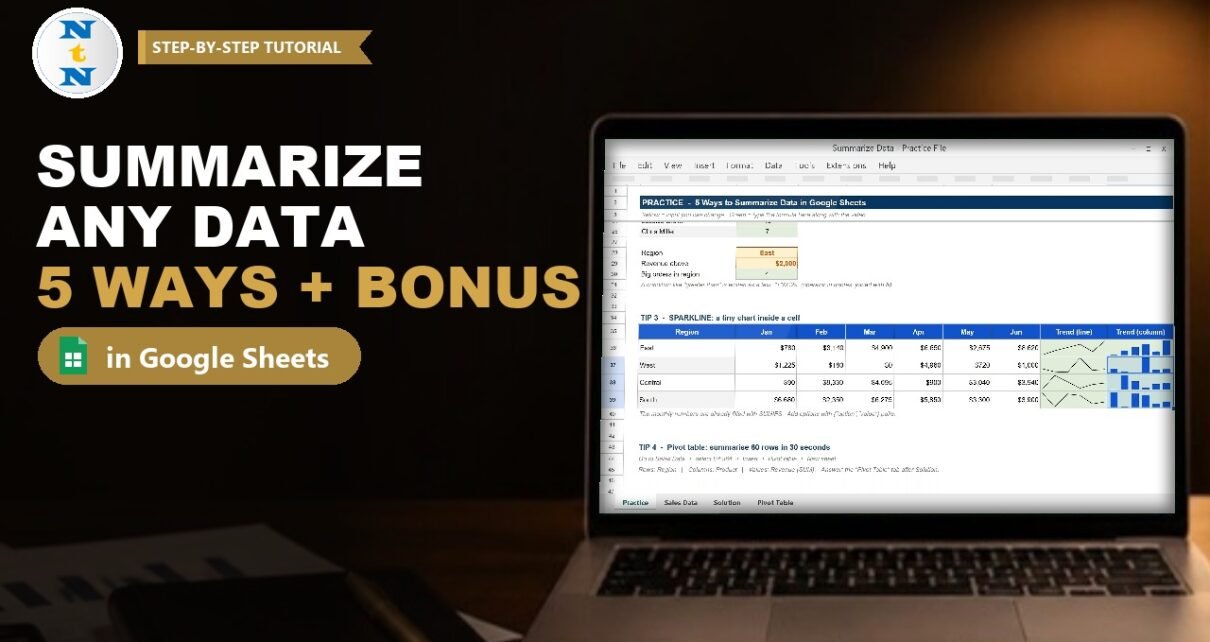
The 10-minute video builds every summary on screen, slowly and one step at a time. It starts with 60 sales orders from January to June 2026, six salespeople and four regions. Tip by tip, the green cells on the Practice sheet fill in: SUMIFS totals the revenue by region, COUNTIFS counts the orders per salesperson, SPARKLINE draws a tiny chart for every region inside a single cell, a pivot table summarizes revenue by region and product in a few clicks, and QUERY builds a sorted summary table from one formula. The bonus shows the status bar, which gives you a sum, an average or a count without typing anything. The chapters are listed below the video on YouTube.
What you will learn
- SUMIFS: add up numbers for the rows that match one or more conditions
- COUNTIFS: count rows, including a condition like “above $2,000”
- SPARKLINE: a line or column chart inside a single cell
- Pivot table: summarize a whole table without writing a formula
- QUERY: a sorted summary table, with a where filter, from one formula
- Bonus: the status bar: an instant sum, average or count
The practice file
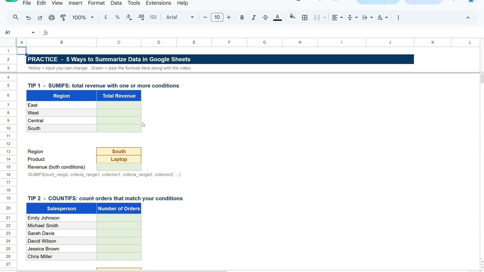
The file has five sheets. Sales Data holds 60 orders with the date, month, region, salesperson, product, units, unit price and revenue. Practice is where you work, Solution has every formula already written, Pivot Table has the finished pivot, and Read Me explains each tip. On the Practice sheet the yellow cells are inputs you can change and the green cells are empty. That is where you type the formulas.
Tip 1: Add up revenue by region with SUMIFS
SUMIFS adds up numbers, but only for the rows that match your condition. The first question is: what is the total revenue for each region?
Step 1: Build the formula with whole-column references
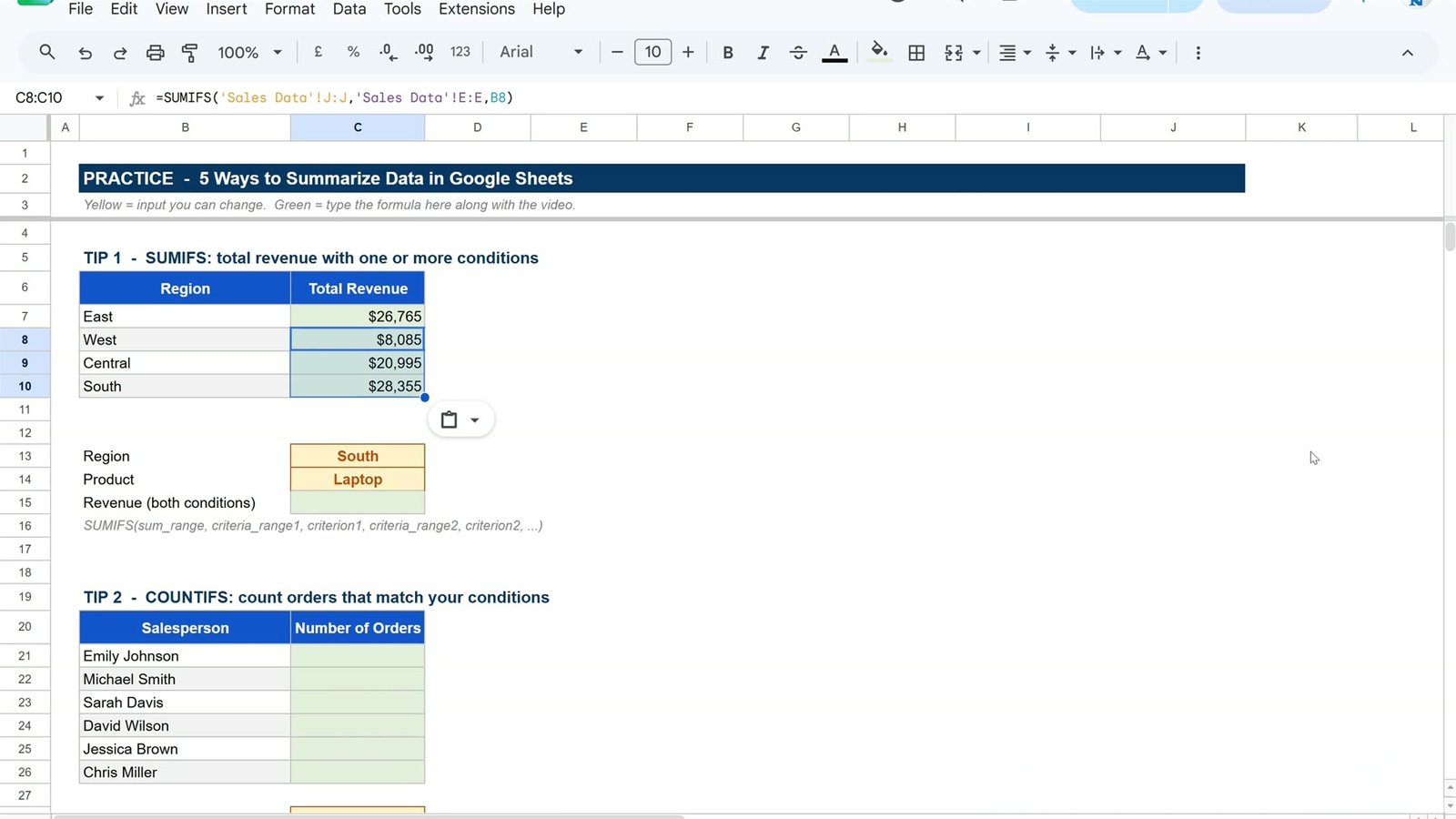
Click C7, type =SUMIFS(, then go to the Sales Data sheet and click the column letter J (Revenue). Type a comma, click column E (Region), type a comma, go back to the Practice sheet and click B7 (East). Close the bracket and press Enter.
=SUMIFS('Sales Data'!J:J,'Sales Data'!E:E,B7)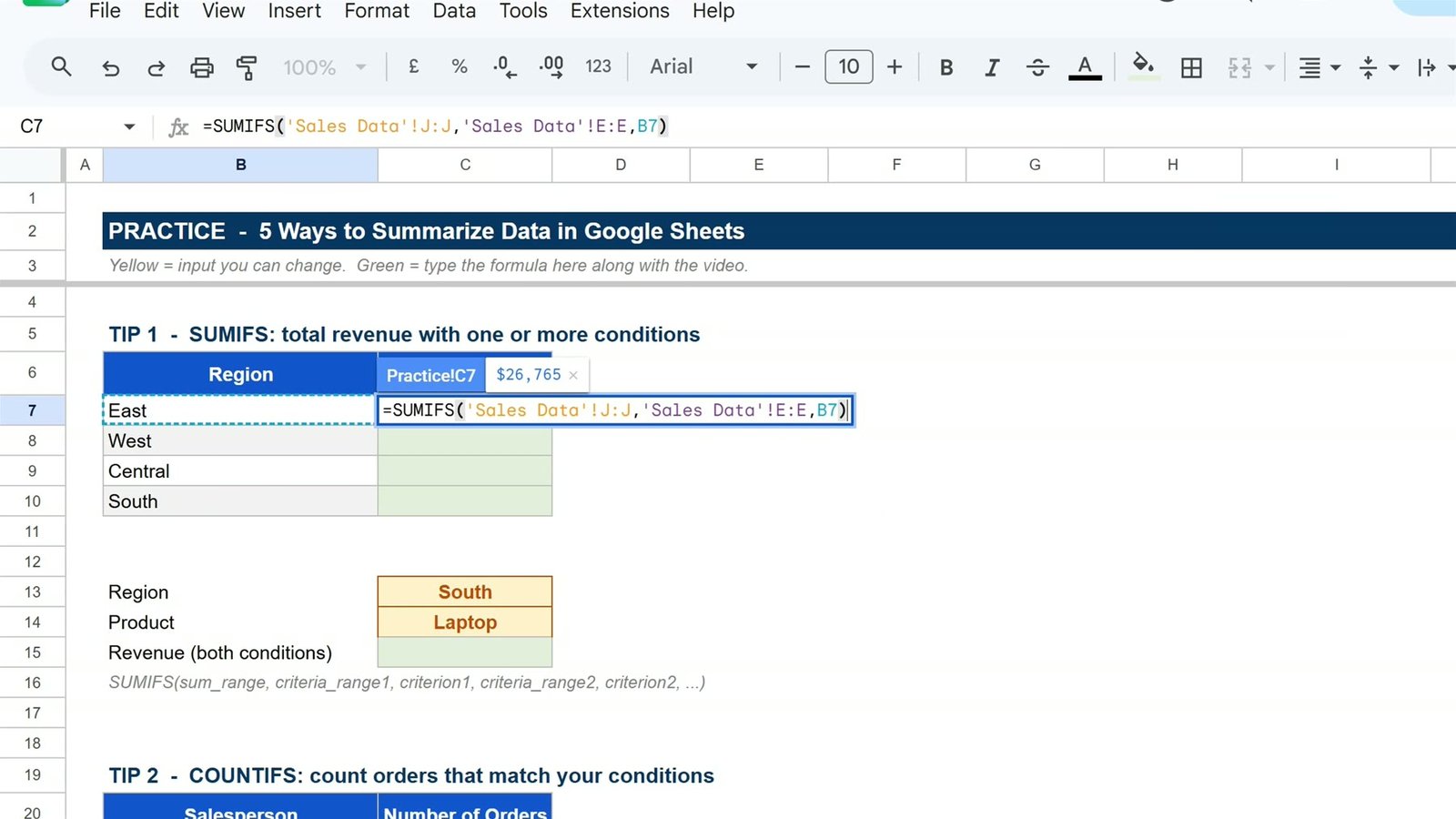
Whole-column references like J:J need no dollar signs, so the formula copies down without breaking, and it keeps working when new orders are added.
Step 2: Copy it down
The East total is $26,765. Copy C7 and paste it into C8:C10. South is the top region with $28,355, then Central ($20,995) and West ($8,085).
Step 3: Two conditions at once
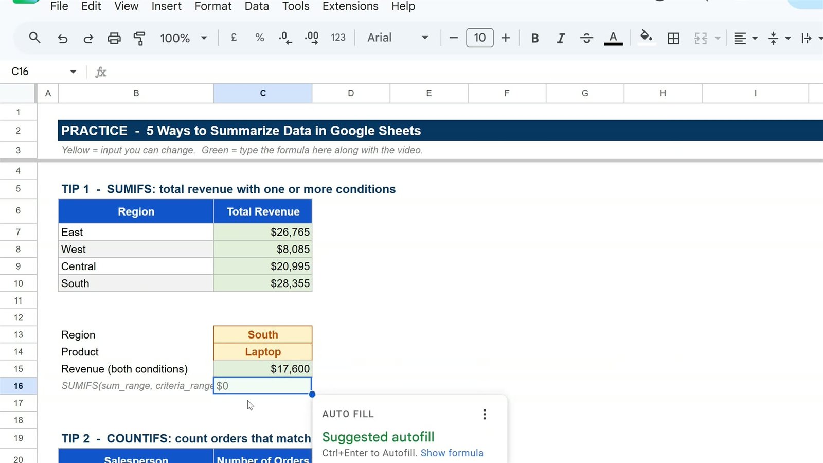
SUMIFS takes more than one condition. For the revenue of the South, but only for laptops, add a second range and criterion pair:
=SUMIFS('Sales Data'!J:J,'Sales Data'!E:E,C13,'Sales Data'!G:G,C14)The answer is $17,600. Change the product in C14 from Laptop to Monitor and it updates by itself to $7,560.
Tip 2: Count orders with COUNTIFS
SUMIFS adds things up; COUNTIFS counts them. How many orders did each salesperson close? Click C21 and type:
=COUNTIFS('Sales Data'!F:F,B21)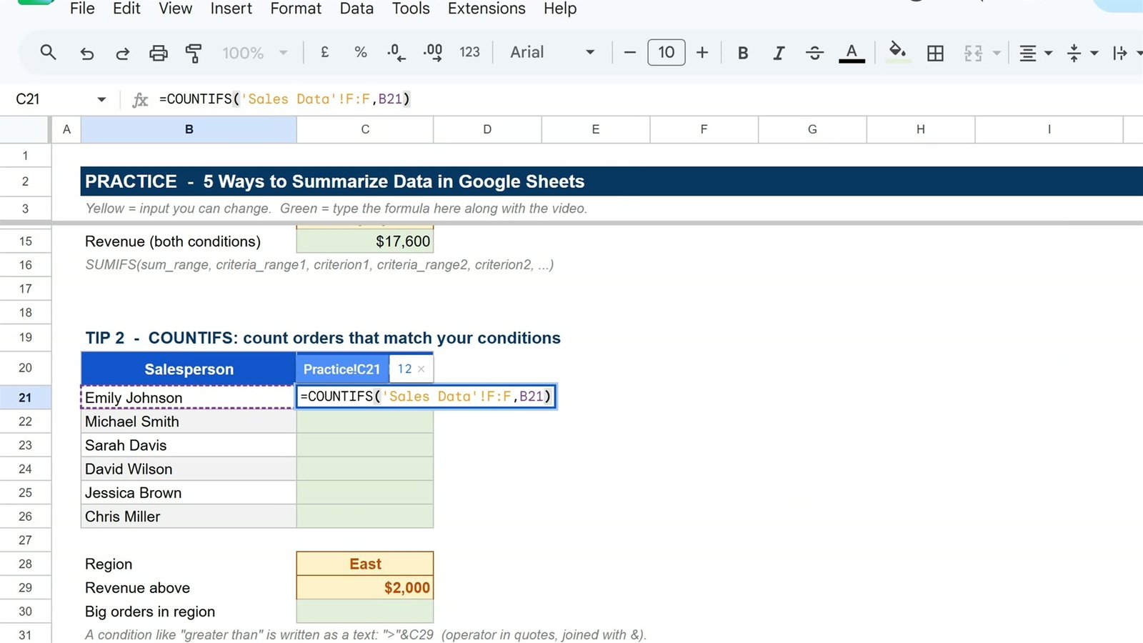
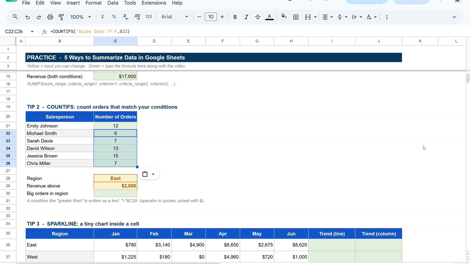
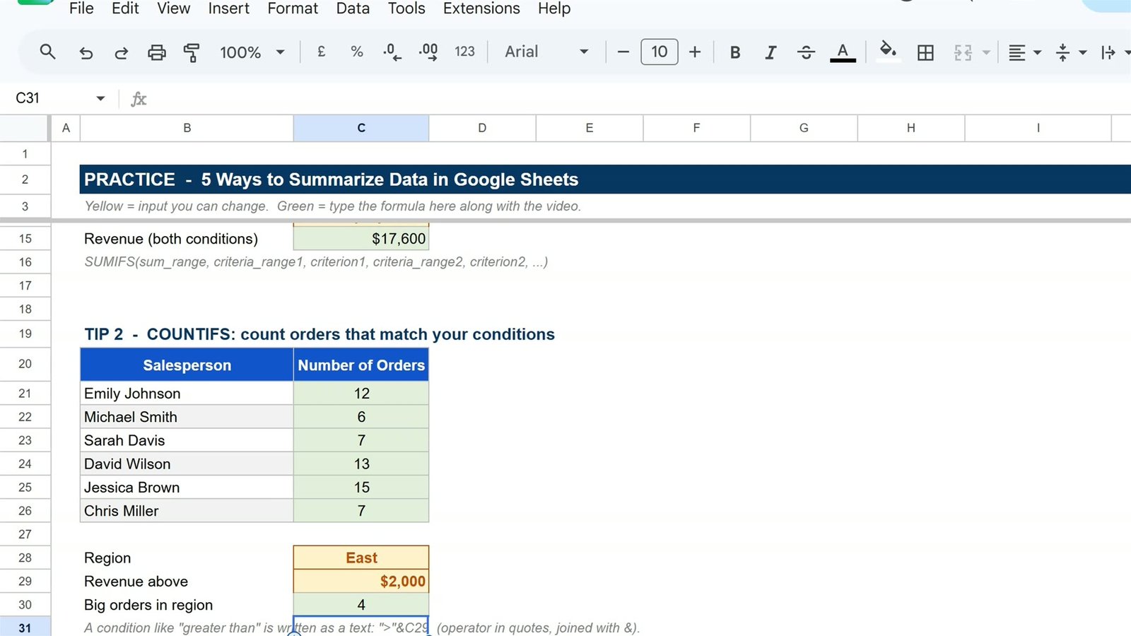
Emily Johnson has 12 orders. Copy it down to all six salespeople: Jessica Brown has the most with 15, and David Wilson is next with 13.
A condition with a number
How many orders in the East were above $2,000? The comparison sign goes inside quotes, and you join it to the cell with the & sign:
=COUNTIFS('Sales Data'!E:E,C28,'Sales Data'!J:J,">"&C29)The answer is 4 big orders in the East.
Tip 3: A chart inside a cell with SPARKLINE
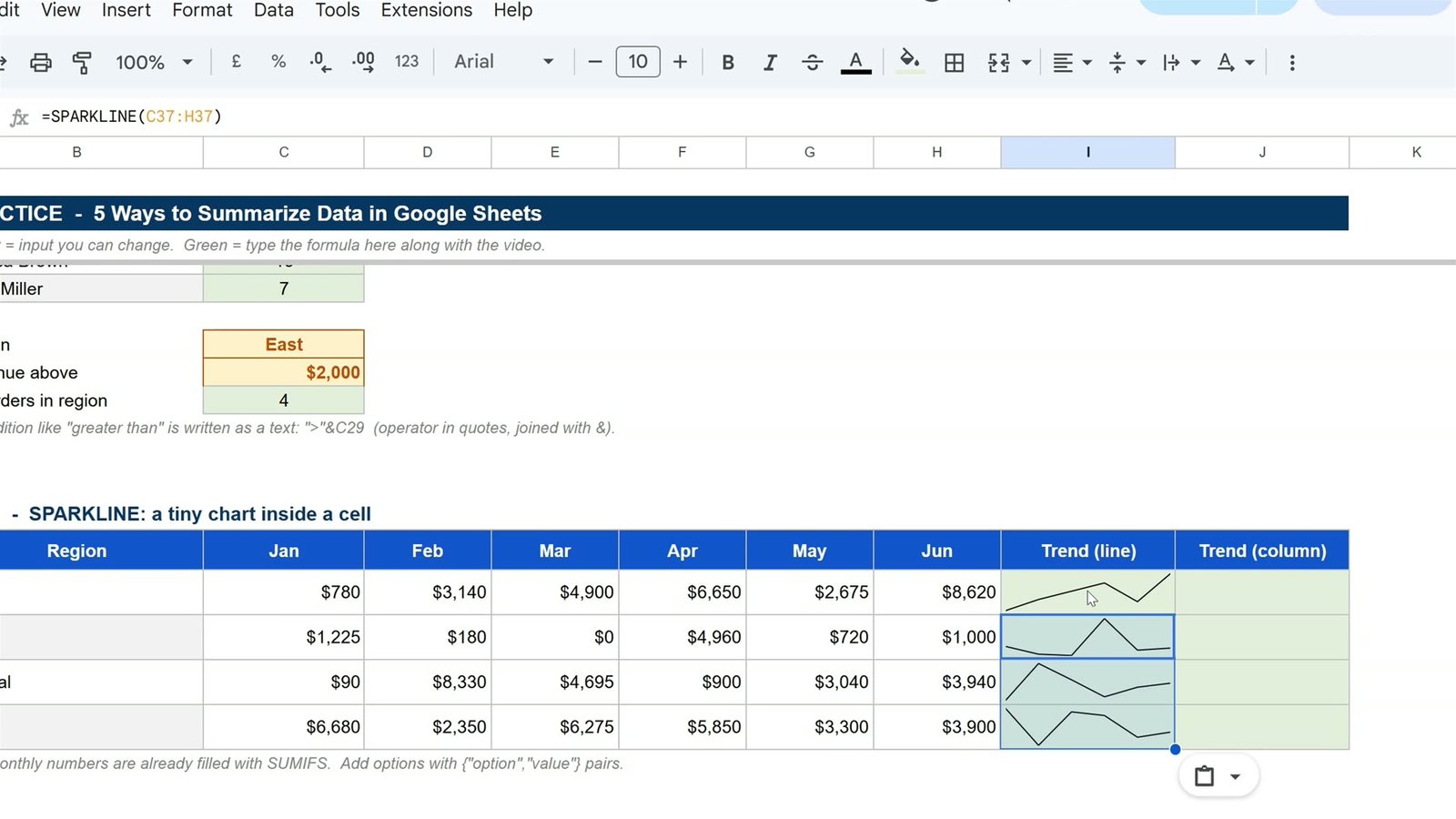
The Practice sheet has the monthly revenue of each region from January to June (already calculated with SUMIFS). From the numbers alone it is hard to see which region is growing. Click I36 and type:
=SPARKLINE(C36:H36)Copy it down to the other regions. The East line climbs from $780 in January to $8,620 in June.
Change the chart type
Options go in curly brackets as name and value pairs. For bars in your own colour:
=SPARKLINE(C36:H36,{"charttype","column";"color","#1155cc"})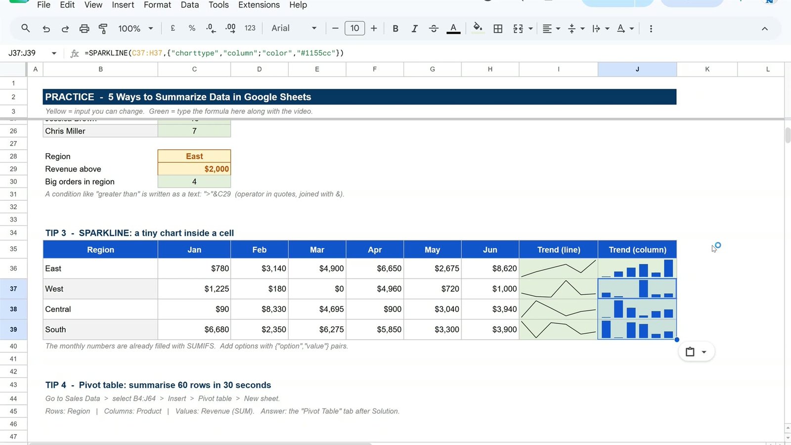
Tip 4: Summarize without formulas using a pivot table
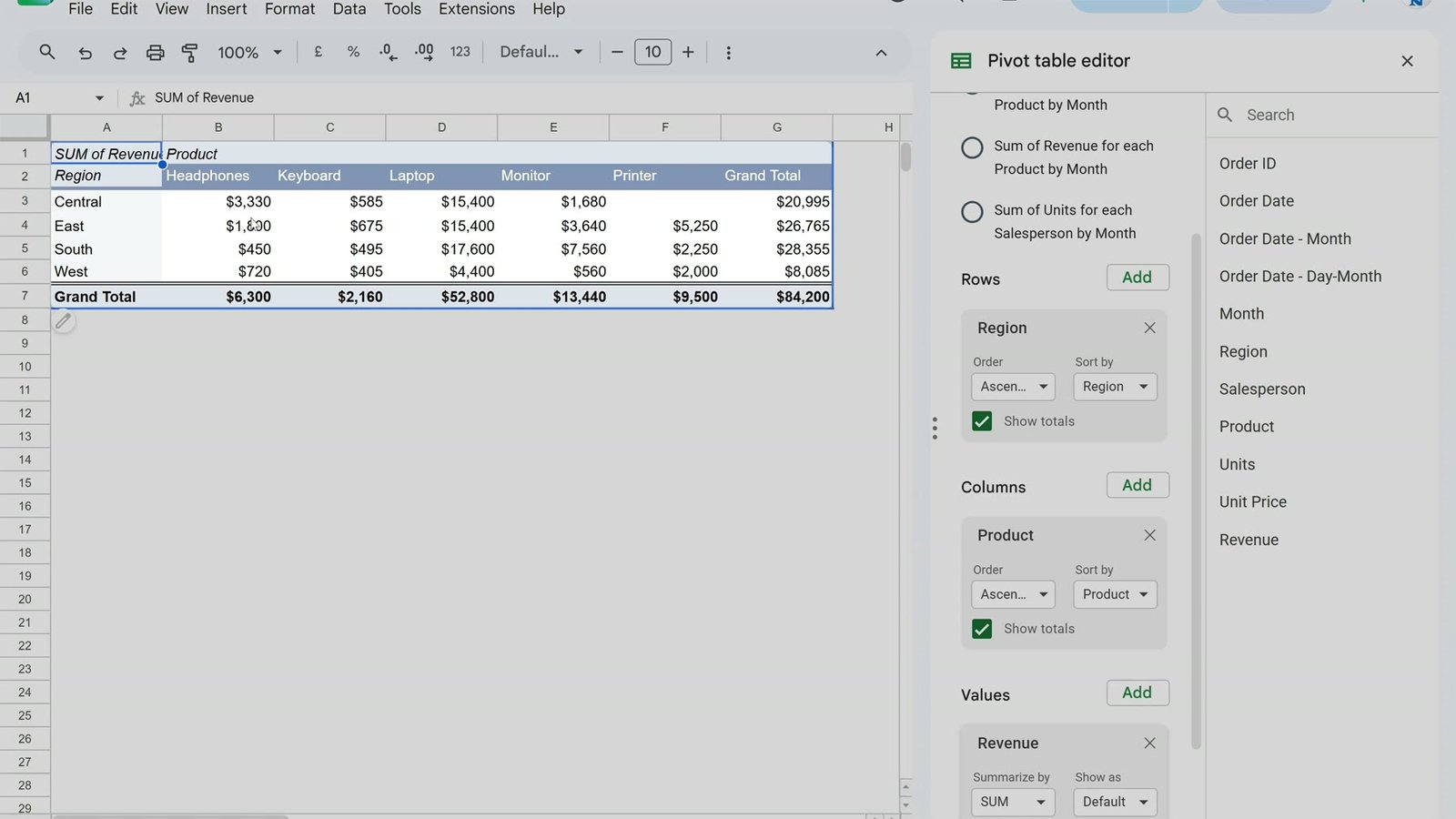
Go to the Sales Data sheet, click any cell inside the data, then Insert > Pivot table. Google Sheets picks up the whole data range. Keep New sheet and click Create.
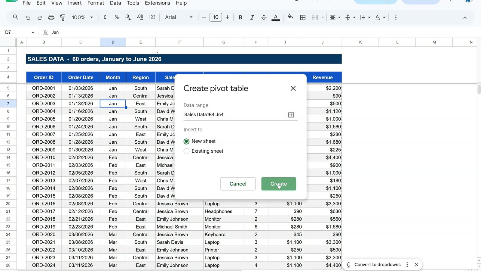
In the pivot table editor: Rows > Add > Region, Columns > Add > Product, and Values > Add > Revenue (summarized by SUM automatically).
Tip 5: A sorted summary table with QUERY
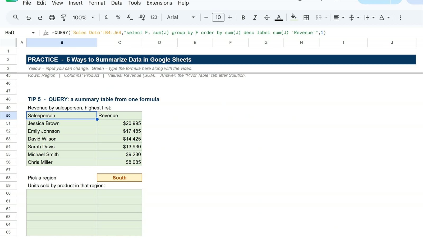
QUERY reads almost like plain English. Click B50, type =QUERY(, go to Sales Data, click B4 and type :J64 (the whole table with headers), then the query in double quotes and a 1 for the one header row:
=QUERY('Sales Data'!B4:J64,"select F, sum(J) group by F order by sum(J) desc label sum(J) 'Revenue'",1)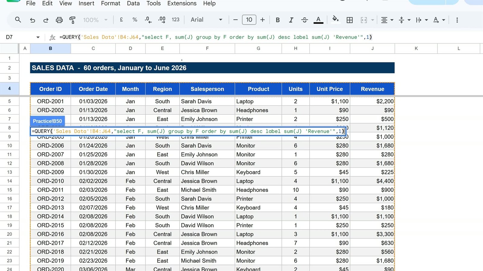
One formula returns the complete summary, sorted from highest to lowest. Jessica Brown is at the top with $20,995.
Filter with a where condition
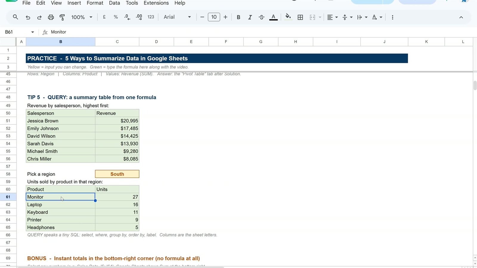
Pick a region in C58, then use it inside the query. Text in QUERY needs single quotes, so the cell is joined between them:
=QUERY('Sales Data'!B4:J64,"select G, sum(H) where E = '"&C58&"' group by G order by sum(H) desc label sum(H) 'Units'",1)In the South, Monitors are the top seller with 27 units.
Bonus: Instant totals in the status bar
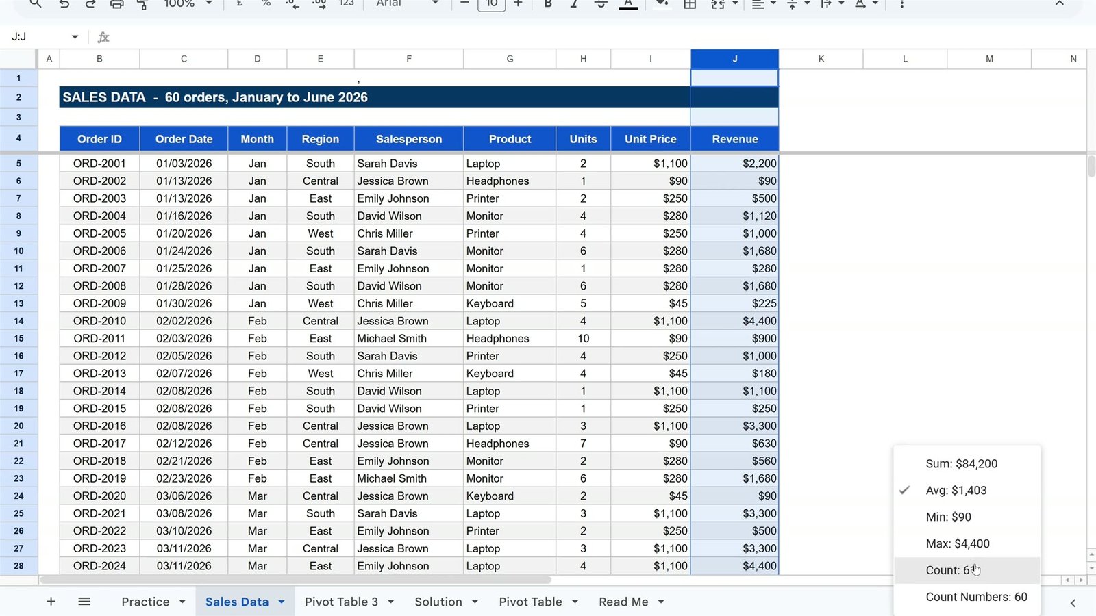
Need a quick total without typing anything? On the Sales Data sheet click the column letter J. The bottom-right corner already shows the sum, $84,200. Click it to switch to the average, minimum, maximum or count. The average is about $1,400 per order.
Cheat sheet
| Question | Tool | Formula / steps |
|---|---|---|
| Total for each group | SUMIFS | =SUMIFS('Sales Data'!J:J,'Sales Data'!E:E,B7) |
| How many rows match | COUNTIFS | =COUNTIFS('Sales Data'!F:F,B21) |
| Rows above an amount | COUNTIFS | =COUNTIFS(...,'Sales Data'!J:J,">"&C29) |
| Trend in one cell | SPARKLINE | =SPARKLINE(C36:H36) |
| Summary with no formula | Pivot table | Insert > Pivot table > Rows, Columns, Values |
| Sorted summary table | QUERY | select F, sum(J) group by F order by sum(J) desc |
| Quick total | Status bar | Select the column, read the bottom-right corner |
Ready to turn summaries like these into full reports? The Excel Pivot Tables & Dashboards course on NextGenTemplates Academy takes the same summarizing ideas further, with practice files.
Frequently asked questions
What is the difference between SUMIF and SUMIFS?
SUMIF takes one condition and puts the sum range last. SUMIFS takes one or more conditions and puts the sum range first. Using SUMIFS every time keeps the order the same.
Why use whole-column references like J:J?
They need no dollar signs, copy down without breaking, and include new rows automatically.
How do I use “greater than” in COUNTIFS with a cell?
Put the sign in quotes and join the cell with &: ">"&C29.
Does a pivot table update when the data changes?
Yes. Google Sheets pivot tables recalculate automatically when the source data changes.
Why does my QUERY return #VALUE or an empty result?
Check that the column letters match the range, that text values are in single quotes inside the double-quoted query, and that the last argument matches the number of header rows.
Can the status bar show more than one total at once?
It shows one at a time, but clicking it opens a list with Sum, Average, Min, Max, Count and Count Numbers.
Written by PK, NeoTech Navigators: step-by-step Google Sheets and Excel tutorials with free practice files.
Download the free practice file
Everything in one page: the view-only Google Sheets link, a one-click Make a copy link, and the full formula cheat sheet from this tutorial.
Free · No sign-up · Opens the Google Sheet in view-only mode, then copy it to your own Drive