If you’re new to Google Sheets or just want to make your work more efficient, you’re in the right place! In this post, I’ll explain two incredibly useful functions—TEXT AND MONTH FUNCTION—that can help you work with dates more easily. These functions allow you to extract specific information from dates, like the day of the week or the month number. Sounds great, right? Let’s dive into how you can use these functions with a simple example!
What Are the TEXT ,MONTH Functions?
Before jumping into the example, let’s take a moment to understand these functions in a simple way:
- TEXT Function: This function lets you format numbers, including dates, as text. For instance, you can take a date like “25-May-2024” and use the TEXT function to display only the day of the week (like “Saturday”).
- MONTH Function: This one is even easier! It extracts the month from a date and returns the month number (like 1 for January, 2 for February, and so on).
Now that we know what these functions do, let’s look at how they work with some real data in Google Sheets.
Step 1: Example Data
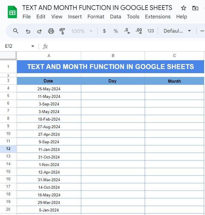
Here’s the data we’ll be working with in Google Sheets. The dates are listed in column A, and we want to figure out the day of the week and month for each date. Here’s how the data looks:
As you can see, we have dates in column A, but nothing yet in the “Day” and “Month” columns. That’s where the TEXT , MONTH functions will come in handy!

Step 2: Using the TEXT Function to Find the Day
First, we’ll use the TEXT function to get the day of the week for each date. Here’s the formula:
=TEXT(A4, "dddd")
How Does the Formula Work?
The TEXT function formats the date in cell A4.
The “dddd” part tells Google Sheets to display the full name of the day, such as “Monday” or “Friday.”
You can enter this formula in column B, right next to the date in column A. The moment you hit enter, the day of the week will appear!
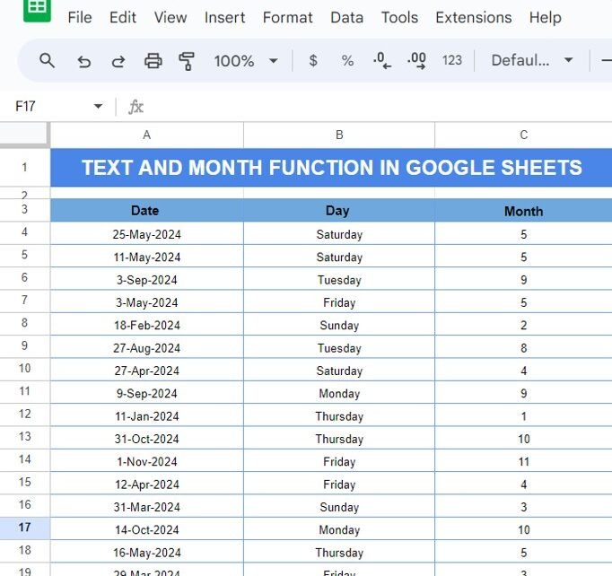
Example Output:
In just a few seconds, you’ve got the day of the week for all your dates!
- Step 3: Using the MONTH Function to Extract the Month
Now, let’s use the MONTH function to extract the month from each date. The formula is super simple:
=MONTH(A4)
How Does This Formula Work?
The MONTH function looks at the date in cell A4 and returns the month number (like 1 for January, 5 for May, etc.).
You can enter this formula in column C, right next to the “Day” column. Once you hit enter, you’ll get the month number for each date!
31-Oct-2024 10
Now you’ve got both the day of the week and the month for each date!
Step 4: Final Results
By combining both the TEXT and MONTH functions, you can easily display both the day and month for each date in your Google Sheets. Here’s how the final table looks:
How easy was that? With just a couple of formulas, you can turn a list of dates into meaningful information about the day of the week and the month.

Why You Should Use TEXT and MONTH Functions
You might be wondering why these functions are so useful. Let me explain a few reasons:
- 🗓️ Custom Date Formats: The TEXT function helps you format dates in a way that makes sense for your needs. Whether it’s showing the day, month, or even year, the TEXT function does it all.
- 📅 Easy Month Extraction: The MONTH function is perfect for pulling out just the month number, which can be helpful when grouping or analyzing data.
- ⚡ Time-Saving: Instead of manually looking up the day or month, these functions get the job done instantly, saving you tons of time.
Conclusion
Using the TEXT and MONTH functions in Google Sheets can make working with dates so much easier. Whether you’re organizing a calendar, analyzing trends, or just playing around with dates, these functions are must-haves in your Google Sheets toolbox.
Visit our YouTube channel to learn step-by-step video tutorials
Youtube.com/@NeotechNavigators
View this post on Instagram
Click here to Make the copy of this Template


