Google Sheets is packed with Powerful Formula Combinations for Google Sheets, but the real magic happens when you combine multiple formulas to create smart, automated workflows. In this guide, you’ll learn 10 powerful formula combinations that will boost your productivity and simplify complex tasks.
Powerful Formula Combinations for Google Sheets
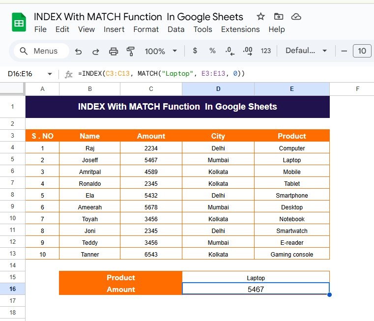
INDEX + MATCH for Advanced Lookups
Say goodbye to VLOOKUP limitations—this combo is faster and more flexible!
Example: Find an Employee’s Salary Based on Their ID
=INDEX(B2:B100, MATCH(E2, A2:A100, 0))
- MATCH(E2, A2:A100, 0) finds the row number for E2 (Employee ID).
- INDEX(B2:B100, row_number) retrieves the salary from column B.
ARRAYFORMULA + IF for Bulk Calculations
Save time by applying calculations to an entire column automatically.
Example: Apply a 10% Discount to Prices Above $100
=ARRAYFORMULA(IF(A2:A100 > 100, A2:A100 * 0.9, A2:A100))
QUERY + IMPORTRANGE for Cross-Sheet Data Analysis
Retrieve filtered and structured data from another Google Sheets file.
Example: Get Total Sales for “Product A” from Another Spreadsheet
=QUERY(IMPORTRANGE("SpreadsheetURL", "Sheet1!A:C"), "SELECT Col1, SUM(Col3) WHERE Col2 = 'Product A' GROUP BY Col1")
TEXTJOIN + FILTER for Smart Data Consolidation
Combine multiple values into one cell based on a condition.
Example: List All Employees in the Marketing Department
=TEXTJOIN(", ", TRUE, FILTER(A2:A100, B2:B100 = "Marketing"))
GOOGLETRANSLATE + ARRAYFORMULA to Translate Entire Columns
Automate translations for large datasets.
Example: Translate a List of Product Names from English to French
=ARRAYFORMULA(GOOGLETRANSLATE(A2:A100, "en", "fr"))
UNIQUE + COUNTIF to Count Duplicates
Quickly identify duplicate entries in a dataset.
Example: Count How Many Times Each Name Appears in Column A
=ARRAYFORMULA(A2:A100 & " - " & COUNTIF(A2:A100, A2:A100))
SPLIT + TRANSPOSE for Cleaning Data
Break text into separate columns dynamically.
Example: Split a List of Names in A1 by Comma and Arrange Vertically
=TRANSPOSE(SPLIT(A1, ","))
REGEXEXTRACT + REGEXMATCH for Pattern Recognition
Extract specific parts of text using regular expressions.
Example: Extract Numbers from a Mixed String in A2
=REGEXEXTRACT(A2, "\d+")
SEQUENCE + EOMONTH for Auto-Filling Dates
Generate dynamic date lists without manual entry.
Example: Create a List of All Dates in the Current Month
=SEQUENCE(DAY(EOMONTH(TODAY(),0)),1,DATE(YEAR(TODAY()),MONTH(TODAY()),1))
SUBSTITUTE + PROPER for Standardizing Text
Quickly clean up messy text formatting.
Example: Convert Names to Proper Case and Remove Extra Spaces
=ARRAYFORMULA(PROPER(TRIM(SUBSTITUTE(A2:A100, " ", " "))))
Final Thoughts
These 10 formula combinations will help you automate tasks, clean data, and analyze information more efficiently. Try them out and transform your Google Sheets experience!
Visit our YouTube channel to learn step-by-step video tutorials
Youtube.com/@NeotechNavigators
Click here to download this Practice File