Every month the operations manager at Copper Kettle Foodservice Supply, a restaurant supply wholesaler in Nashville, Tennessee, exports the orders and spends a morning with a calculator: who sold what, which deliveries ran late, which orders were biggest. This tutorial turns that morning into 10 Google Sheets formulas for work: SPLIT, XLOOKUP, IFS, NETWORKDAYS, TEXT, UNIQUE, SUMIFS, AVERAGEIFS, COUNTIFS and SORTN. You use all ten on one real sheet, a monthly sales report with 104 orders, a sales rep scorecard and a top 5 orders list. The free practice file has the raw export on the Practice tab and the finished report on the Solution tab.
📥 Download the FREE Practice File (Excel .xlsx)
Offline copy: README, Practice, Solution and Lists tabs
📄 Make Your Own Copy in Google Sheets
Opens a copy in your Google Drive – sign in to Google first
Watch the Video Tutorial
Video Overview
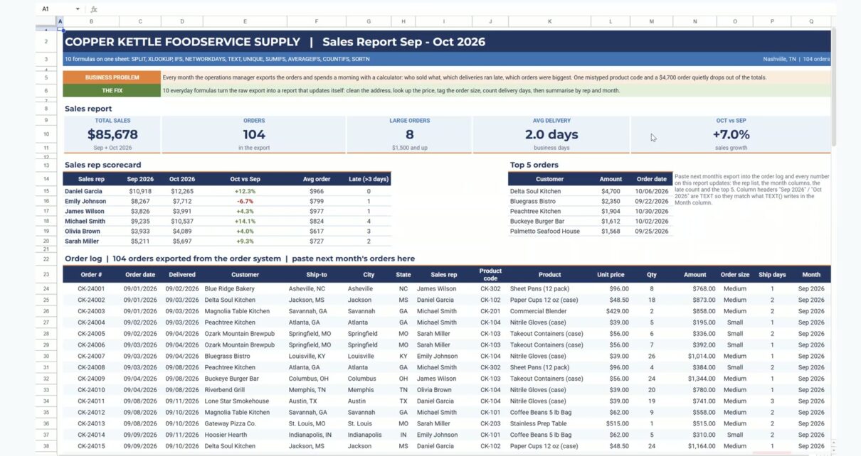
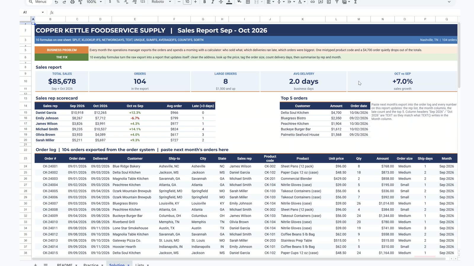
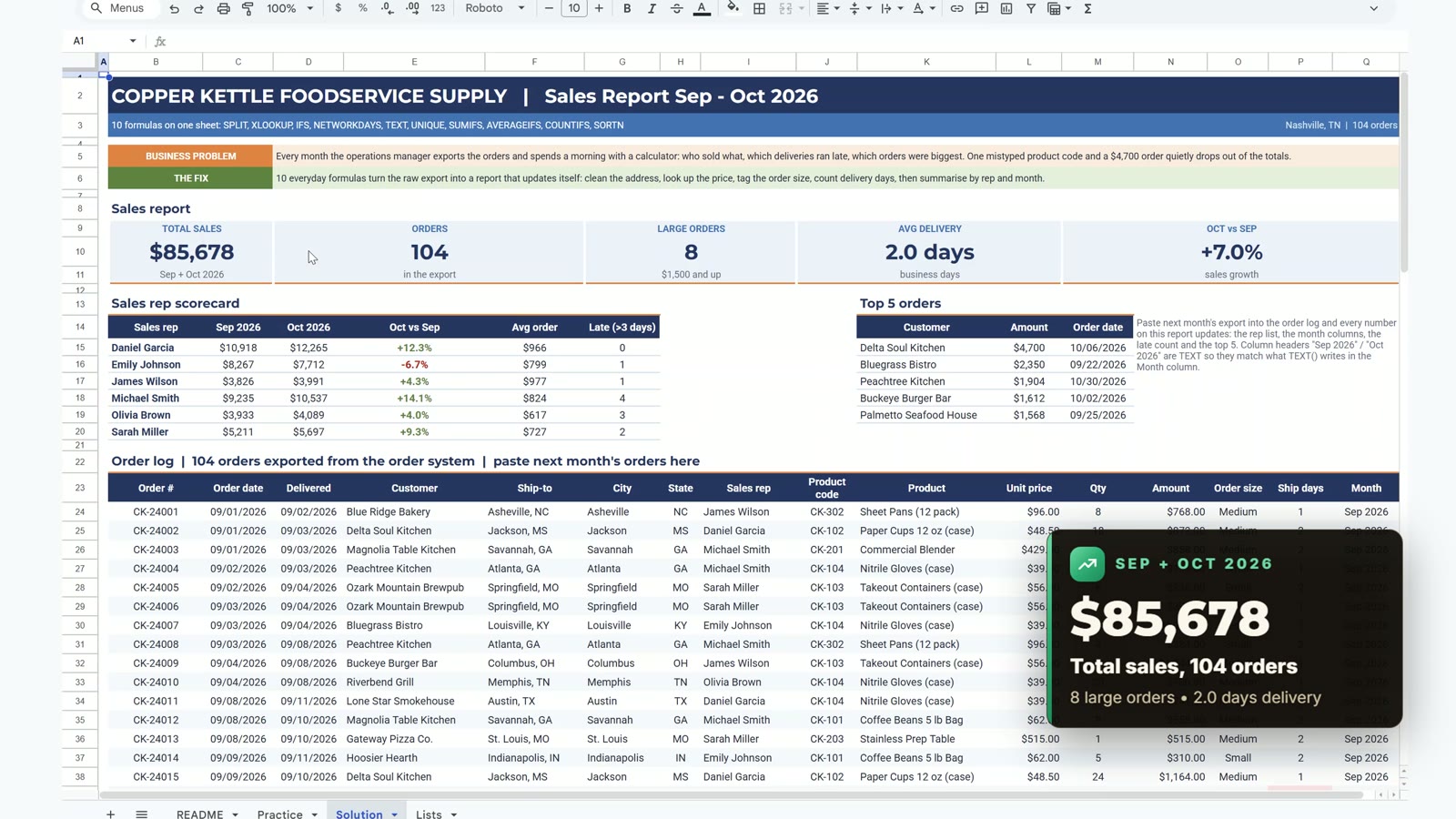
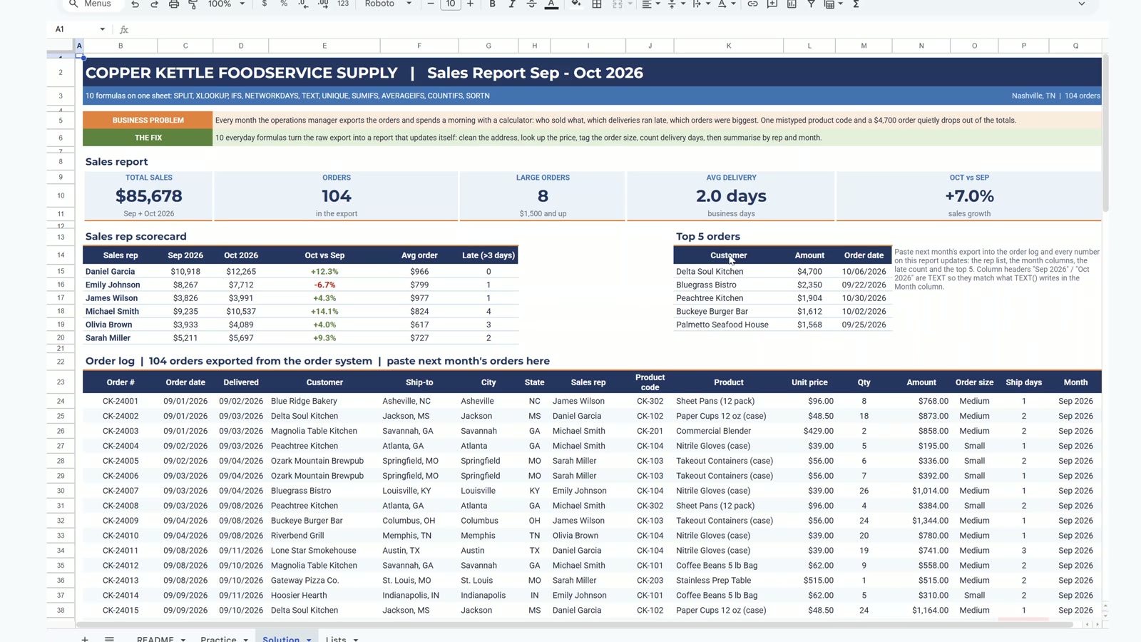
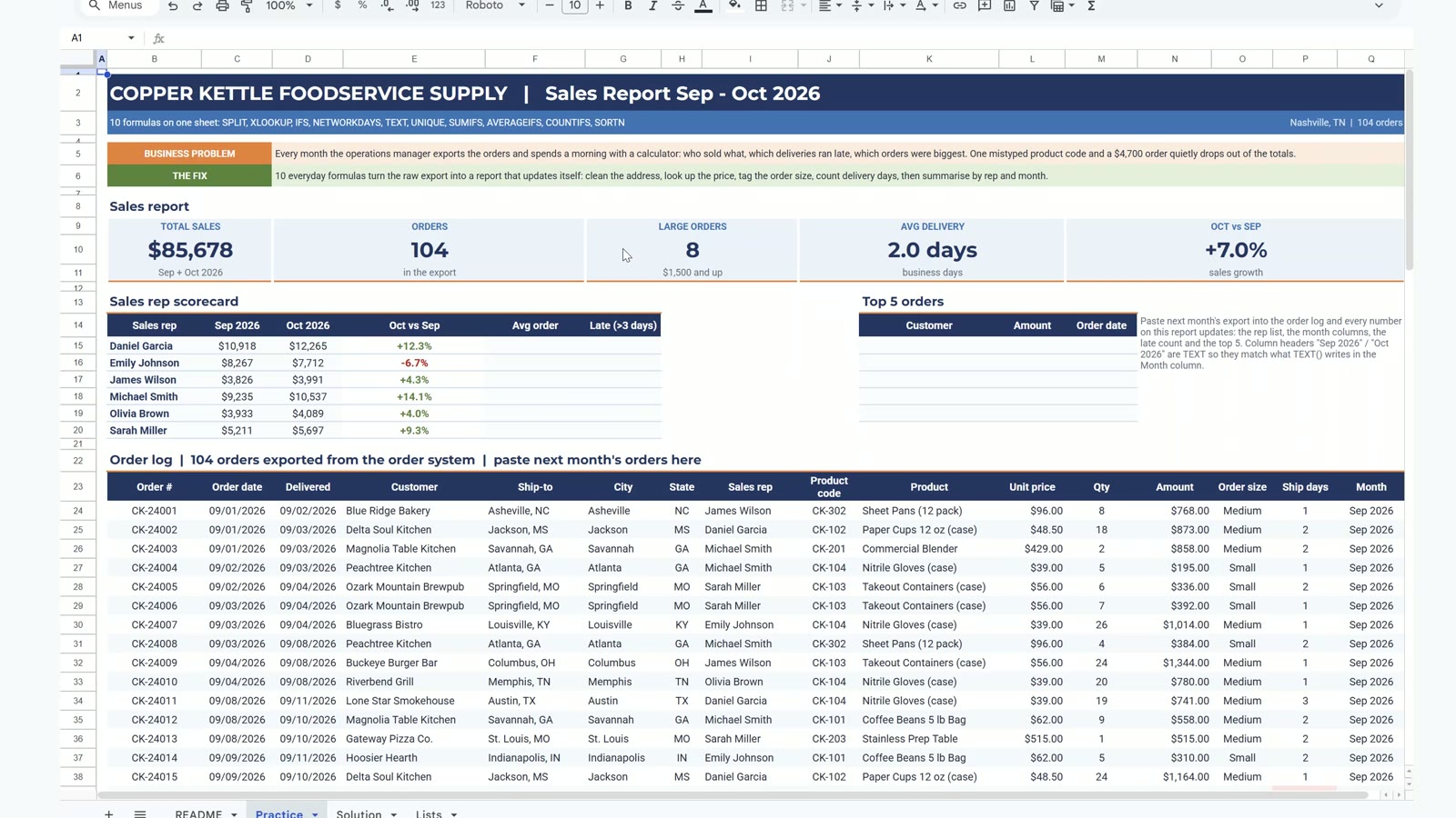
The video opens with the finished report: $85,678 in total sales, 104 orders, 8 large orders, 2.0 days average delivery and October up 7.0% on September. Then you move to the Practice tab and add the ten formulas one by one, about 15 minutes in total. One mistyped product code (CK-2O4 with a letter O) hides a $4,700 order until XLOOKUP flags it, and the fix changes Daniel Garcia from -30.7% to +12.3%. Pause anywhere and follow along with the practice file.
What You Will Build
- Five KPI cards: total sales, orders, large orders, average delivery days and October against September.
- A sales rep scorecard with September and October sales, growth, average order and late deliveries for six reps.
- A top 5 orders list that updates by itself.
- Seven helper columns in the order log: city, state, product, unit price, order size, ship days and month.
The Problem: A Raw Order Export
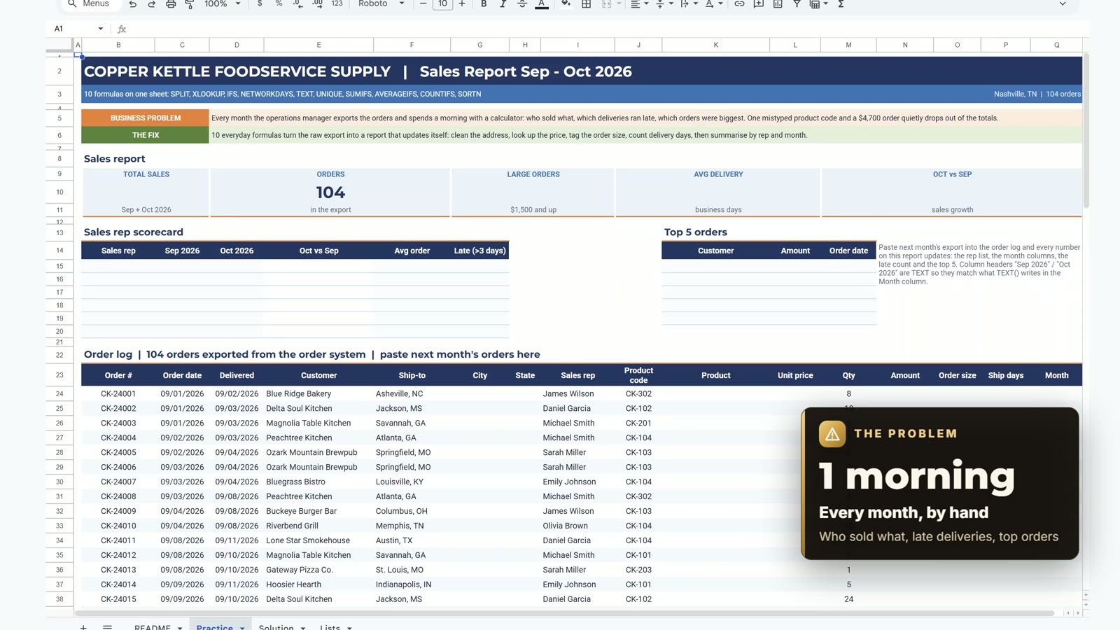
The export has 104 orders from September 1 to October 30, 2026, ten products, fourteen restaurant customers and six sales reps. The ship-to column holds city and state in one cell, the product and price are missing, and nothing is grouped. Start on the Practice tab: the report area is empty and waits for formulas.
Formula 1: SPLIT (City and State)
Select G24 and split the Ship-to text at the comma. Type the default version first and fill it down: row 36, St. Louis, MO, splits into St., Louis and MO and spills into the sales rep column with a #REF! error. The third argument FALSE fixes it by splitting only on the whole comma-and-space, not on each character.
=SPLIT(F24,", ",FALSE)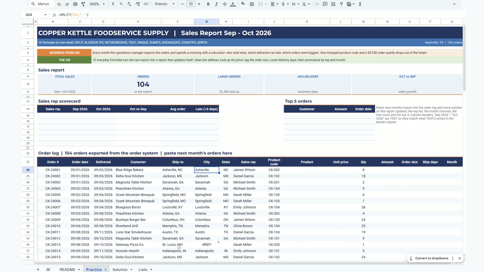
Formula 2: XLOOKUP (Product and Unit Price)
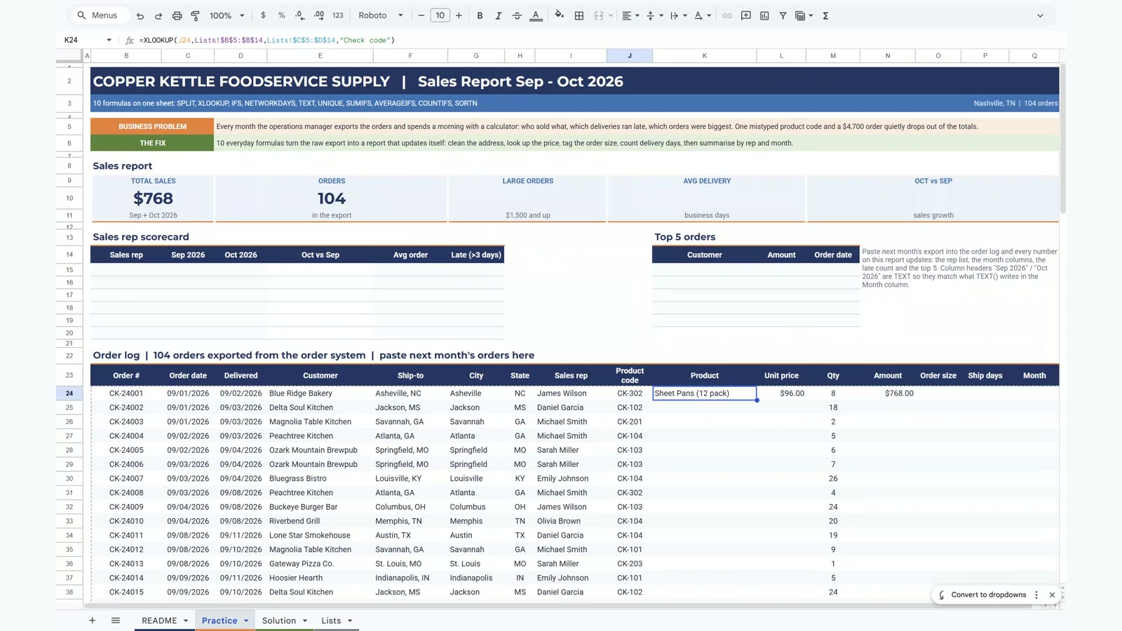
Pull the product name and price from the Lists tab by product code. Because the return range covers two columns, one formula in K24 fills both the Product and the Unit price cells. The fourth argument shows Check code when a code is not found, and the Amount column (quantity times price) lights up.
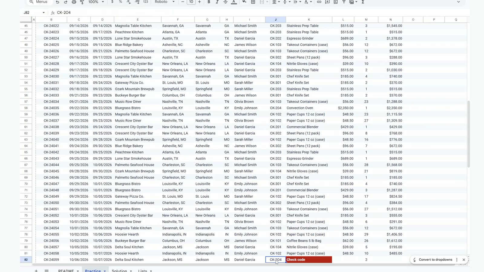
=XLOOKUP(J24,Lists!$B$5:$B$14,Lists!$C$5:$D$14,"Check code")Scroll to row 82 and you see the red Check code: the product code says CK-2O4 with a letter O instead of the zero. Retype it as CK-204 and the row becomes a Convection Oven, $2,350 times 2 = $4,700 for Delta Soul Kitchen on 10/06/2026.
Formula 3: IFS (Order Size)
Label every order Large (1,500 and up), Medium (400 and up) or Small. The empty check keeps blank rows blank, and TRUE as the last test means everything else. Large orders then show as green chips and the card counts them.
=IF(N24="","",IFS(N24>=1500,"Large",N24>=400,"Medium",TRUE,"Small"))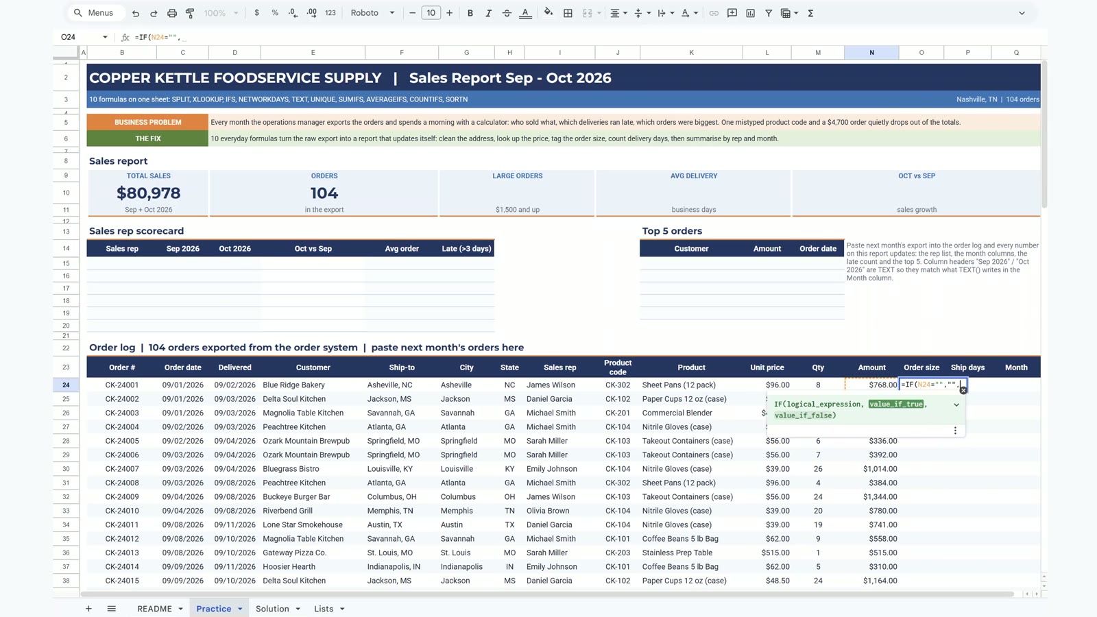
Formula 4: NETWORKDAYS (Ship Days)
Count working days between the order date and the delivery date, skipping the company holidays on the Lists tab. Two details matter: NETWORKDAYS counts both end days, so subtract 1; and orders on 09/03 and 09/04 delivered on 09/08 cross Labor Day, which shows 3, 2 and 2 days without the holiday range but the correct 2, 1 and 1 with it. The average delivery card becomes 2.0 days, and anything above 3 days turns red.
=NETWORKDAYS(C24,D24,Lists!$F$5:$F$7)-1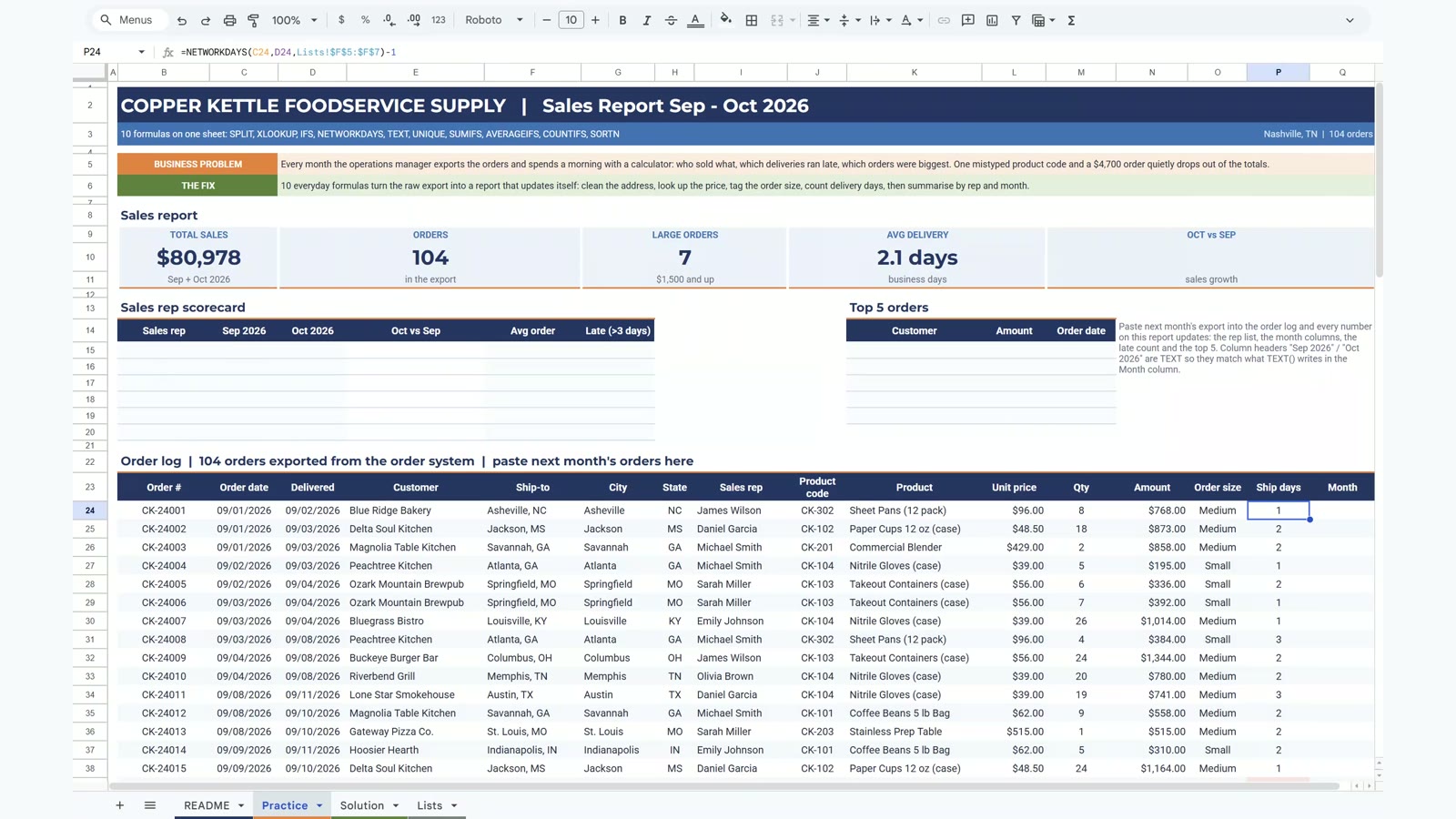
Formula 5: TEXT (Month Label)
Turn the order date into a month label such as Sep 2026. The result is text, so the report headers for September and October must be text as well. If you type Sep 2026 into a normal cell, Sheets converts it to a date and SUMIFS returns 0.
=TEXT(C24,"mmm yyyy")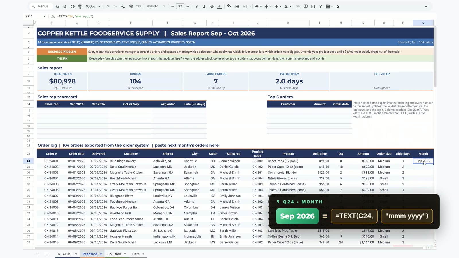
Formula 6: UNIQUE (Sales Rep List)
Build the scorecard rows from the data instead of typing names. UNIQUE returns the six reps, SORT puts them in A to Z order, and a new rep in next month’s export appears automatically.
=SORT(UNIQUE(I24:I127))Formula 7: SUMIFS (Sales by Rep and Month)
This is the formula you will use most. It adds the Amount column for one rep in one month. Fill it right and down: the dollar signs lock the rep column ($B15) and the month header row (C$14), so one formula fills the whole table and the growth column and the Oct vs Sep card come alive.
=SUMIFS($N$24:$N$127,$I$24:$I$127,$B15,$Q$24:$Q$127,C$14)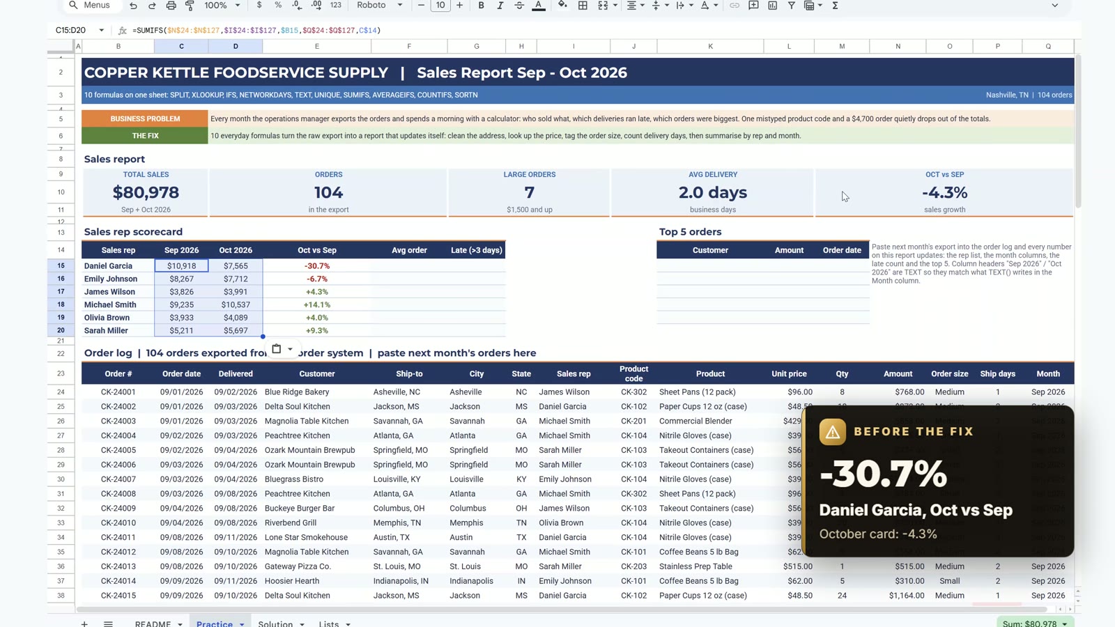
Now the payoff. With CK-2O4 still in the data, Daniel Garcia looks like -30.7% and the card says -4.3%. After the code is fixed to CK-204 the same formulas give +12.3% and +7.0%. A one-character typo changed the story, and XLOOKUP was the formula that caught it.
Formula 8: AVERAGEIFS (Average Order per Rep)
The average order value for each rep, using the same rep criteria as SUMIFS. Daniel Garcia averages $966 and Olivia Brown $617.
=AVERAGEIFS($N$24:$N$127,$I$24:$I$127,$B15)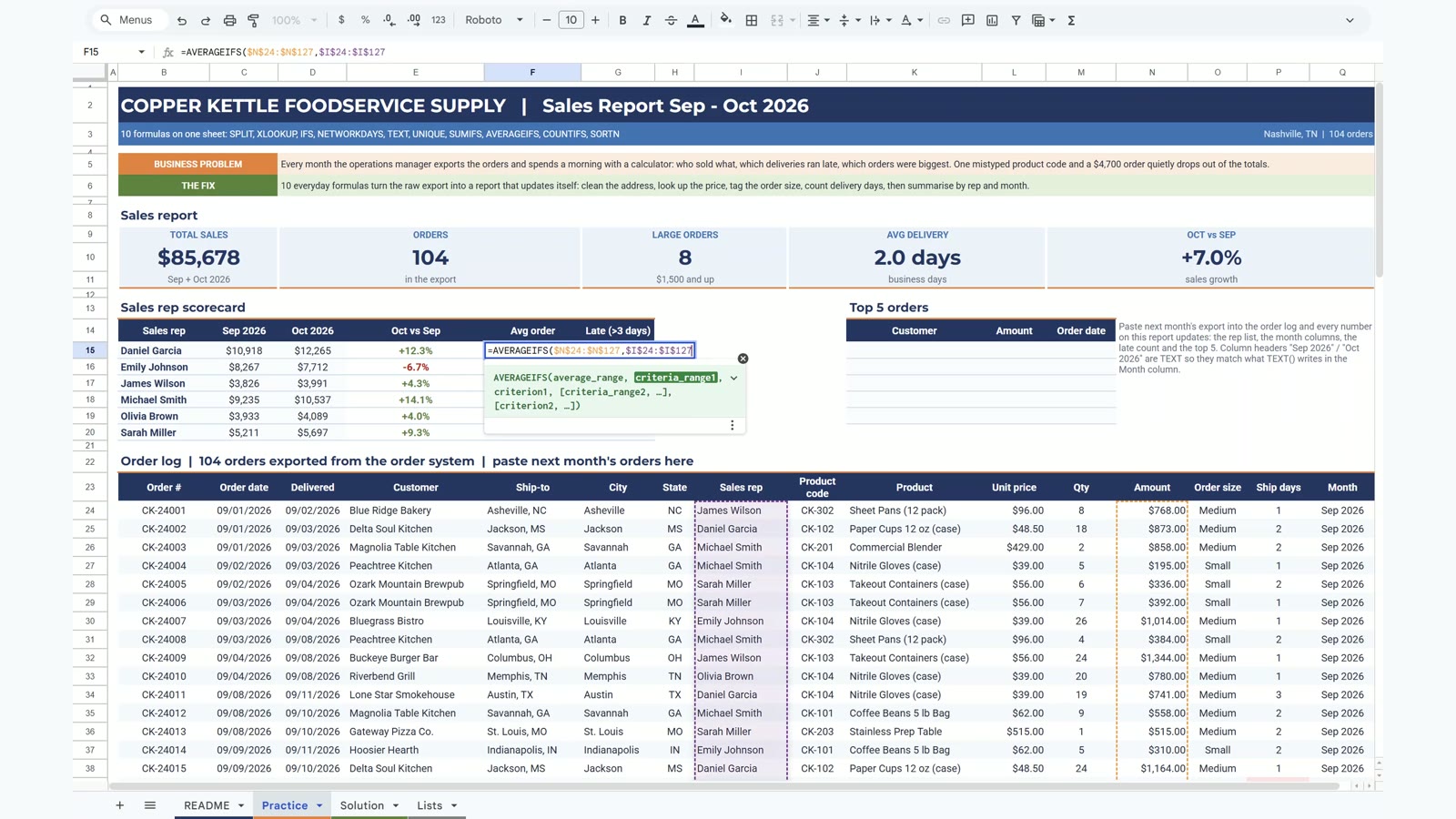
Formula 9: COUNTIFS (Late Deliveries per Rep)
Count the orders that took more than 3 days. The condition goes in quotes: “>3”. Michael Smith has 4 late deliveries, Olivia Brown 3, and Daniel Garcia none.
=COUNTIFS($I$24:$I$127,$B15,$P$24:$P$127,">3")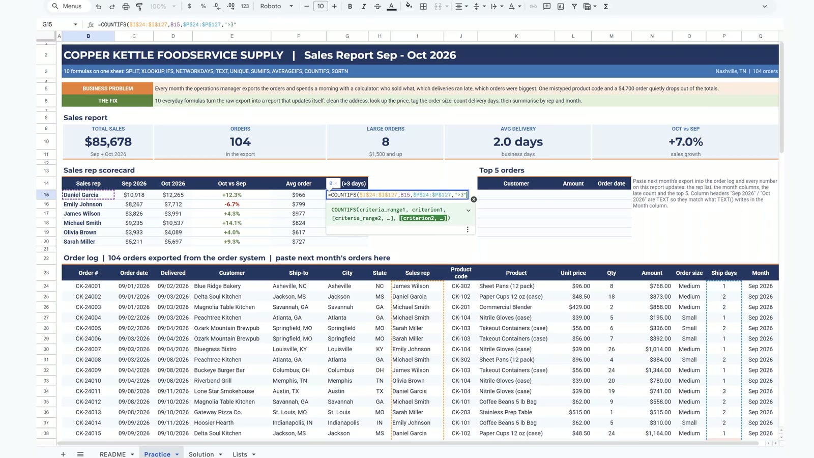
Formula 10: SORTN (Top 5 Orders)
SORTN returns the top rows of a sorted range. The curly brackets build a three-column range of customer, amount and order date; 5 is the number of rows, and sorting on column 2 descending gives the biggest orders: Delta Soul Kitchen $4,700, Bluegrass Bistro $2,350, Peachtree Kitchen $1,904, Buckeye Burger Bar $1,612 and Palmetto Seafood House $1,568.
=SORTN({E24:E127,N24:N127,C24:C127},5,0,2,FALSE)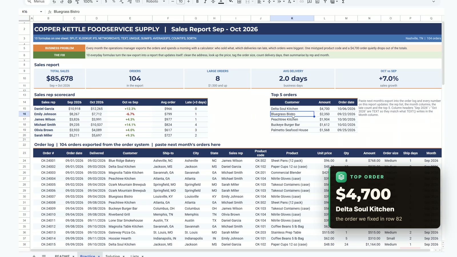
Use These Google Sheets Formulas on Your Own Data
Next month, paste the new export into the order log and the whole report updates by itself. Swap in your own products on the Lists tab and your own holidays, keep the column order, and compare with the Solution tab if a result looks off. The Excel download is an offline copy for reading the layout; the Google Sheets copy keeps every formula working.
📥 Download the FREE Practice File (Excel .xlsx)
Offline copy: README, Practice, Solution and Lists tabs
📄 Make Your Own Copy in Google Sheets
Opens a copy in your Google Drive – sign in to Google first
Want a Ready-Made Sales Report?
If you want a sales report that does even more, look at the Monthly Sales Tracker and Report in Google Sheets from Next Gen Templates. To learn Sheets step by step, see the Google Sheets Course: Beginner to Advanced on Next Gen Templates Academy.
🛒 Get the Monthly Sales Tracker and Report
Google Sheets · Next Gen Templates
Related Google Sheets Tutorials
- 9 Google Sheets Tricks for Business Reports
- Google Sheets ARRAYFORMULA: Stop Dragging Formulas Down
- Invoice Template in Google Sheets
The official Google Docs Editors function list explains every argument of these formulas.
Frequently Asked Questions
Which Google Sheets formulas are used most at work?
For business reports the workhorses are SUMIFS, COUNTIFS and AVERAGEIFS for totals by group, XLOOKUP to pull a price or name from a list, IFS to label rows, and TEXT, SPLIT and UNIQUE to clean and group the data. This tutorial uses all of them on one sales report.
Why does SPLIT break a city name like St. Louis?
By default SPLIT cuts on every character in the delimiter, so ", " cuts on the comma and on the space. St. Louis, MO becomes three pieces and spills into the next column. Adding FALSE as the third argument tells SPLIT to cut only on the whole comma-plus-space.
How can XLOOKUP return two columns at once?
Point the return range at two columns, such as Lists!$C$5:$D$14, and type the formula in one cell. The result spills into the cell next to it, so one formula brings back the product name and the unit price.
Why do I subtract 1 from NETWORKDAYS?
NETWORKDAYS counts both the start day and the end day. An order delivered the next day would show 2 working days, so subtracting 1 gives the days between the two dates. The holiday range makes it skip company holidays such as Labor Day.
Why is the Sep 2026 header in the report text and not a date?
Typing Sep 2026 in a normal cell turns it into a date, and SUMIFS then finds no match and returns 0. TEXT(C24,"mmm yyyy") returns text, so the log column and the report headers match exactly.
What do the dollar signs in the SUMIFS formula do?
$B15 locks the rep column while the row changes, and C$14 locks the month header row while the column changes. One formula then fills the whole rep by month table.
Will this report update when I add next month's orders?
Yes. Paste the new export into the order log and the formulas fill in the city, product, size, shipping days and month, and the scorecard and cards update by themselves.
More Google Sheets tutorials are on the NeoTech Navigators blog and the YouTube playlist.