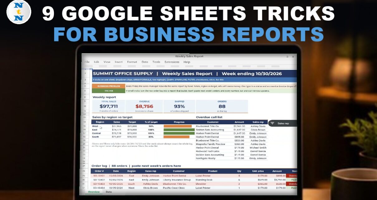
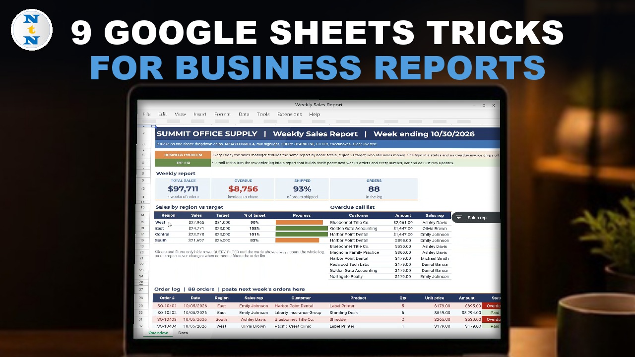
Every Friday the sales manager rebuilds the same report by hand: totals, region against target and who still owes money. These 9 Google Sheets tricks turn a raw order log into a weekly sales report that builds itself. You paste next week’s orders and every number, bar and call-list row updates. The sample business is Summit Office Supply in Denver with 88 orders, 8 reps and 4 regions. Formulas and built-in features only.
⬇️ Download the Free Practice File
Google Sheets · opens a Make a copy page · Practice + Solution sheets · no add-ons
Watch the Video Tutorial
Video Overview
The 16-minute video starts with a 90-second look at the finished report, then builds it trick by trick on the Practice sheet: dropdown chips, ARRAYFORMULA, a whole row highlight, QUERY, SPARKLINE bars, a FILTER and SORT call list, checkboxes, a slicer and a live title. A bonus adds an Apps Script button that stamps a reminder date on every overdue row.
9 Google Sheets Tricks for Business Reports: What You Will Build
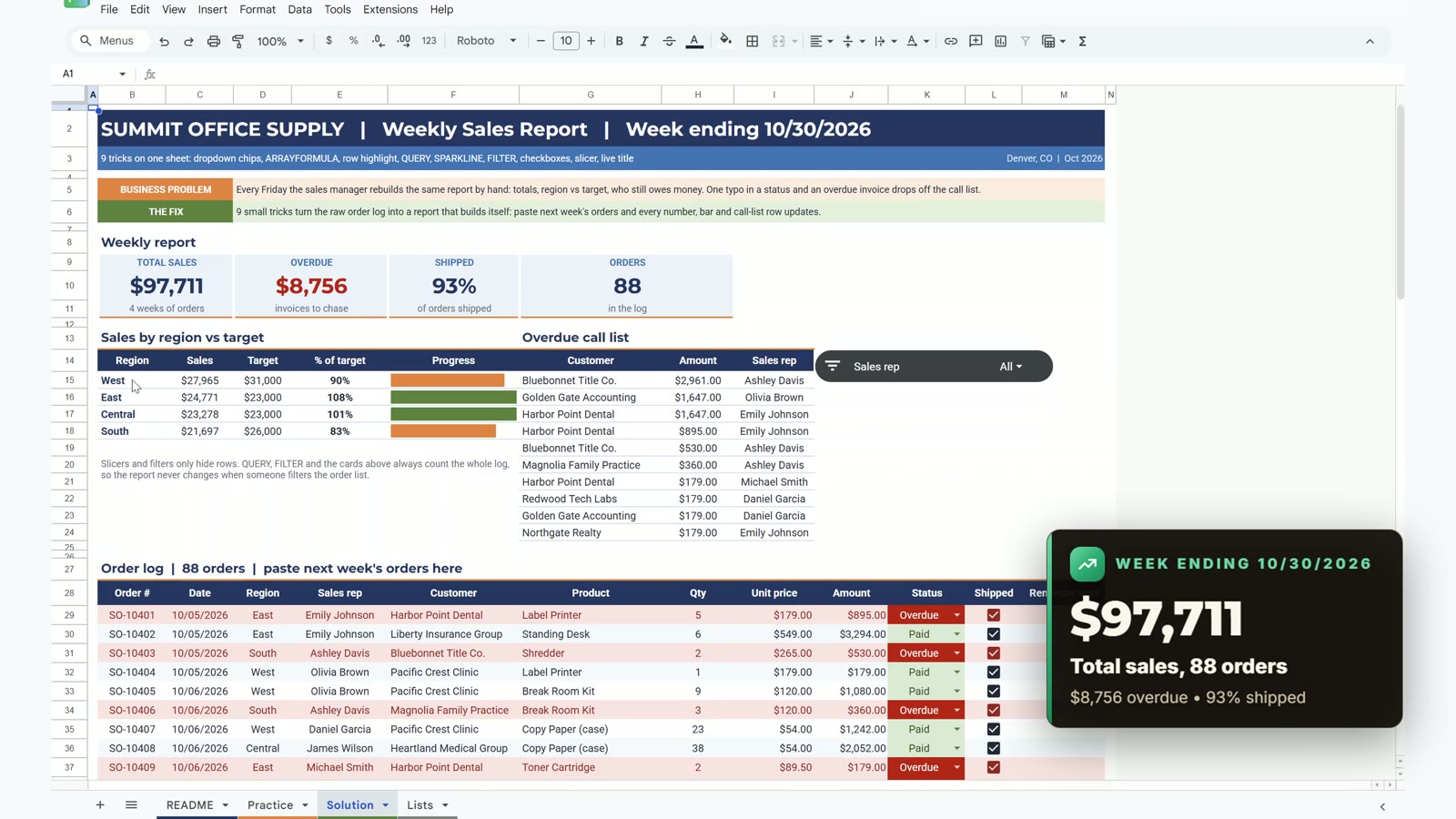
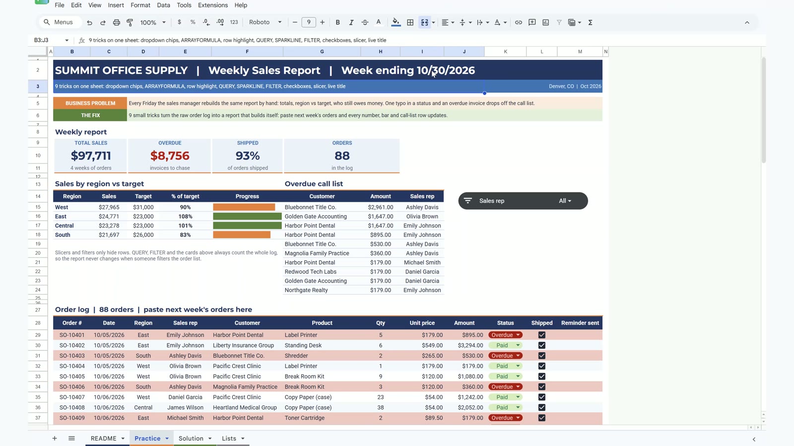
- Report cards for total sales ($97,711), overdue ($8,756), shipped (93%) and orders (88).
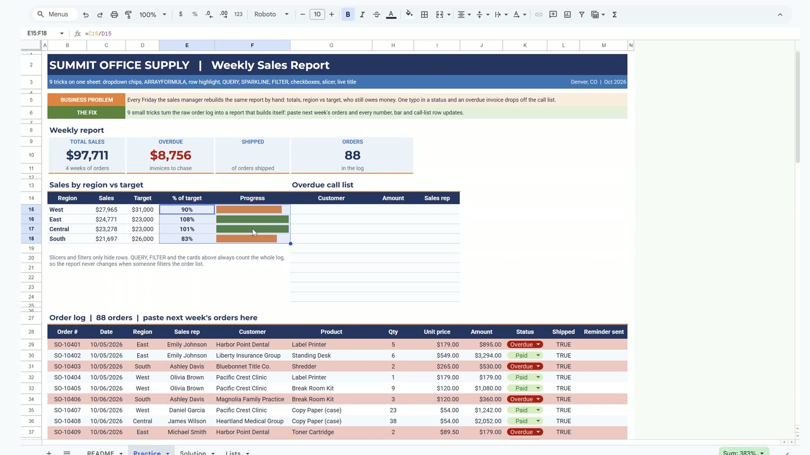
- Sales by region against target with progress bars: West 90%, East 108%, Central 101%, South 83%.
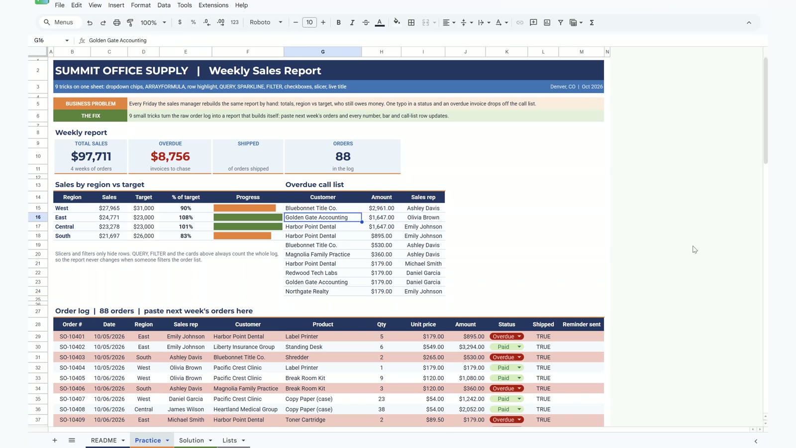
- An overdue call list sorted biggest first, led by Bluebonnet Title Co. at $2,961.
- A live title that always shows the week ending date.
The Practice File
The free file opens a Make a copy page. It has a README, the Practice sheet to build along with the video, the finished Solution sheet and a Lists sheet with the October targets. The order log has 88 orders from 10/05 to 10/30/2026.
Trick 1: Dropdown Chips for Status
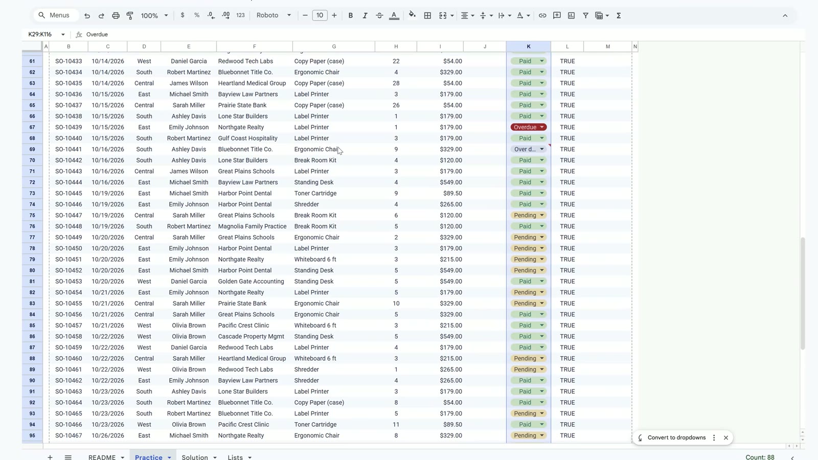
Select K29:K116, choose Insert, then Dropdown, and add Paid, Pending and Overdue with green, yellow and red colours. Under Advanced options choose Reject the input. Now every status is a coloured chip. One row said Over due; pick Overdue and the biggest overdue invoice ($2,961) is counted by the call list in trick 6.
Trick 2: ARRAYFORMULA for the Whole Amount Column
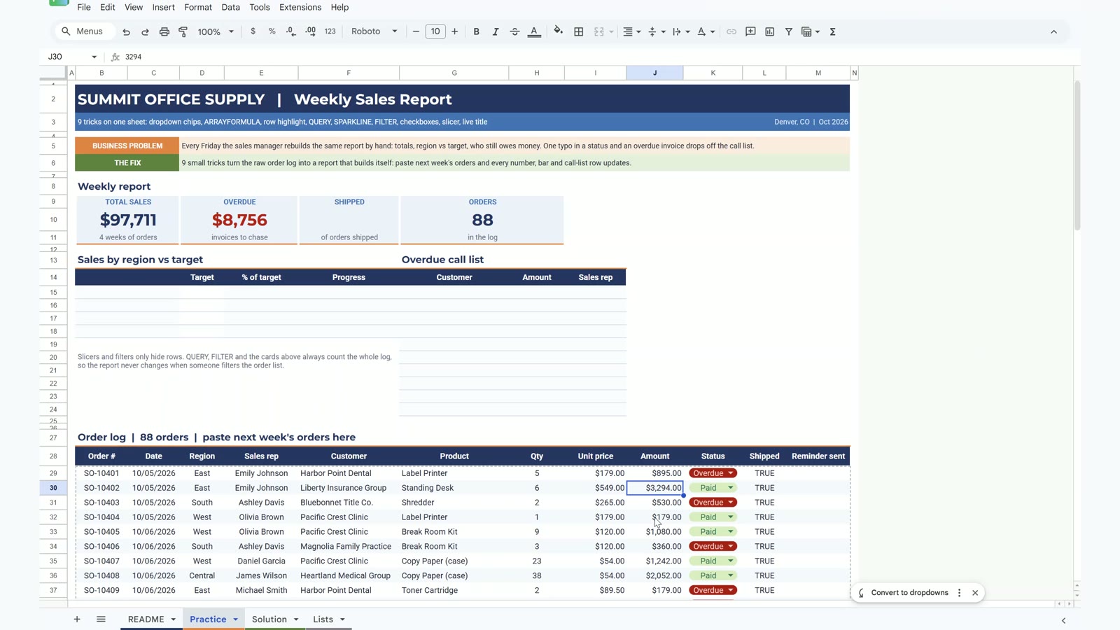
In J29 type one formula for all 88 rows. The IF keeps empty rows blank.
=ARRAYFORMULA(IF(H29:H116="","",H29:H116*I29:I116))The cards light up: $97,711 in sales, $8,756 overdue and 88 orders.
Trick 3: Highlight the Whole Row, Not One Cell
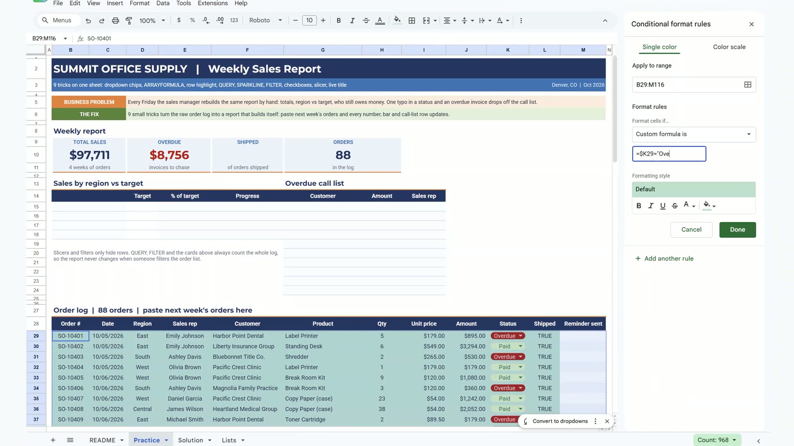
Select B29:M116, open Format, then Conditional formatting, choose Custom formula is and type:
=$K29="Overdue"The dollar sign before K is what makes the whole row follow column K. Pick a light red fill.
Trick 4: QUERY for Sales by Region
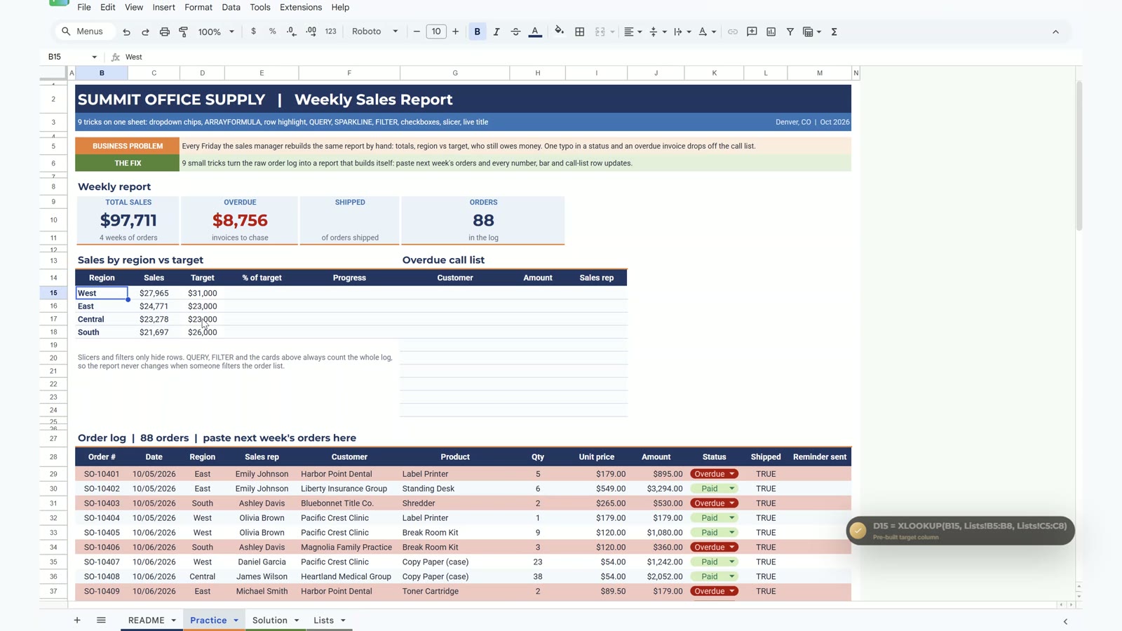
In B14 type:
=QUERY(B28:M116,"select D, sum(J) where B is not null group by D order by sum(J) desc label sum(J) 'Sales'",1)QUERY uses the column letters of the range, so D is Region and J is Amount. It needs empty cells to spill into.
Trick 5: SPARKLINE Progress Bars
In E15 divide sales by target, then in F15 draw the bar and copy it down to row 18:
=SPARKLINE(C15,{"charttype","bar";"max",D15;"color1",IF(E15>=1,"#548235","#ED7D31")})Green means the target is met, orange means it is not.
Trick 6: FILTER and SORT for an Overdue Call List
In G15 type:
=SORT(FILTER({F29:F116,J29:J116,E29:E116},K29:K116="Overdue"),2,FALSE)It lists the 10 overdue invoices, biggest first. Trick 1 just saved this list.
Trick 7: Checkboxes
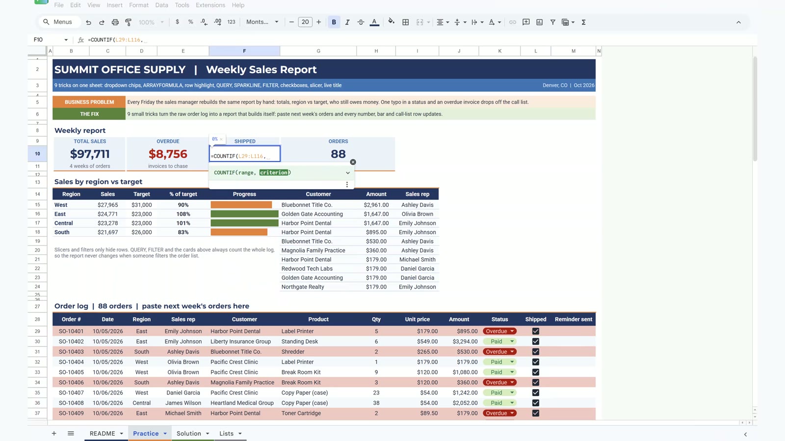
Select L29:L116 and choose Insert, then Checkbox. TRUE and FALSE become ticks. Then F10 shows the shipped percentage:
=COUNTIF(L29:L116,TRUE)/COUNTA(B29:B116)That gives 93% (82 of 88 orders).
Trick 8: A Slicer, and the Gotcha
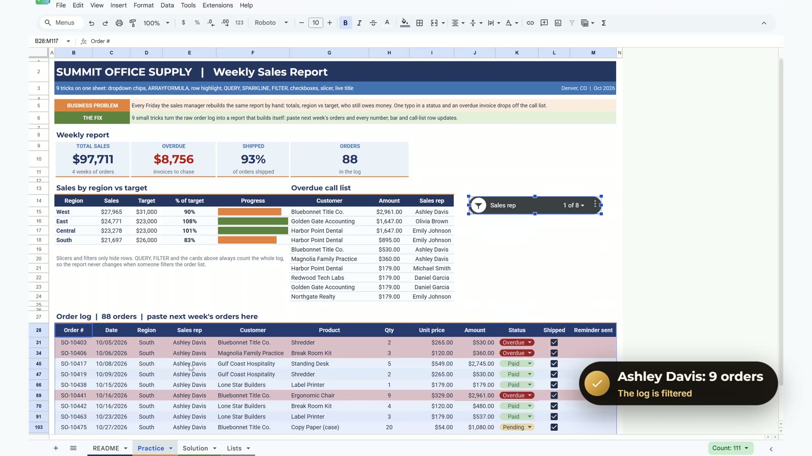
Click in the log, choose Data, then Add a slicer, pick Sales rep and drag the slicer next to the call list. Choose Ashley Davis and the log filters to 9 orders. The gotcha: a slicer only hides rows. QUERY, FILTER and the cards still count the whole log, so the report does not change when someone filters it.
Trick 9: A Live Title
Click the title in B2 and type:
="SUMMIT OFFICE SUPPLY | Weekly Sales Report | Week ending "&TEXT(MAX(C29:C116),"mm/dd/yyyy")Next week’s paste moves the date in the title on its own.
Bonus: An Apps Script Button
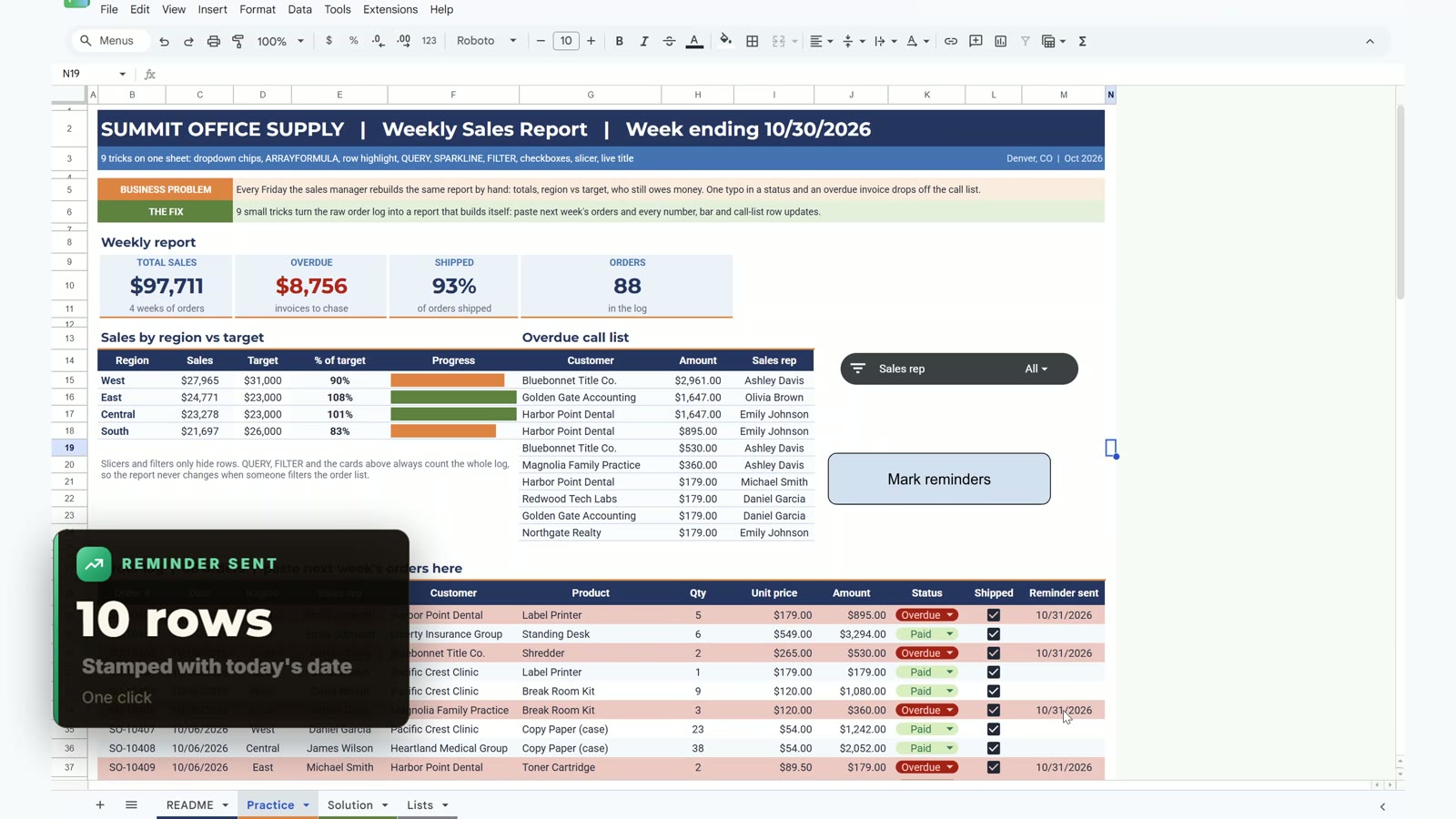
This part is optional. Open Extensions, then Apps Script, paste the markReminders code from the README, save and authorise it. Then insert a drawing called Mark reminders and assign the script. One click stamps today’s date on the 10 overdue rows. Do it on your own copy only.
Want a Ready-Made Sales Dashboard?
If you would rather start from a finished file, see the Sales KPI Dashboard in Google Sheets from Next Gen Templates. Also work in Excel? The Excel + AI Mastery: 100 Essential Formulas and Real-World Projects course teaches the same ideas step by step.
Frequently Asked Questions
How do I build a weekly sales report in Google Sheets that updates itself?
Keep the raw order log on one sheet and put the report on top of it. Use ARRAYFORMULA for the amount column, QUERY for sales by region, SPARKLINE for the progress bars, FILTER and SORT for the overdue call list and a TEXT formula for the title. When next week's orders are pasted in, every number updates.
Is the practice file free?
Yes. The practice file opens a Make a copy page, so you get your own editable Google Sheet with a README, the Practice sheet to build along, the finished Solution sheet and a Lists sheet. All names and numbers are made up for the demo.
What does ARRAYFORMULA do in Google Sheets?
It runs one formula down a whole range, so a single cell fills the entire Amount column. Wrap it in IF so empty rows stay blank: =ARRAYFORMULA(IF(H29:H116="","",H29:H116*I29:I116)).
Why does my QUERY return the wrong column?
QUERY uses the column letters of the range you give it, not the letters of the sheet. In a range that starts at column B, Region is D and Amount is J. QUERY also needs empty cells below and to the right so it can spill.
Does a slicer change my report numbers?
No. A slicer only hides rows. The cards, QUERY and FILTER still count the whole order log, so the report does not change when someone filters the log.
How do I keep a typo in a status from hiding an overdue invoice?
Use dropdown chips with Reject the input turned on. In the demo one row said Over due, so the FILTER call list silently missed the biggest overdue invoice, $2,961. A dropdown makes that typo impossible.
Do I need Apps Script for this report?
No. The nine tricks are formulas and built-in features. The bonus Mark reminders button is the only Apps Script part and it is optional.
Download the Free Practice File
⬇️ Download the Free Practice File
Google Sheets · opens a Make a copy page · Practice + Solution sheets · no add-ons
More Google Sheets tutorials are on the NeoTech Navigators blog and the YouTube playlist.