In this article, we have explained about the new feature Tables in Google Sheets. Now, you can use the Tables in Google Sheet like we use in Microsoft Excel.
Tables in Google Sheets:
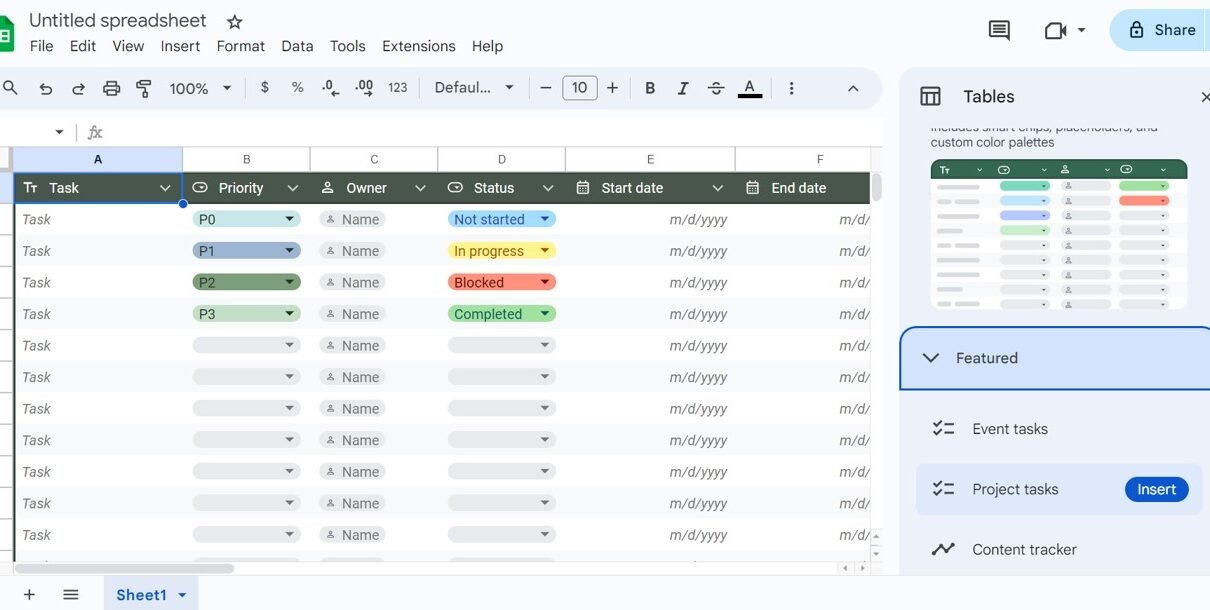
As you create a new sheet in the Google Sheets, I will a new window pane on the Right hand side. You can select any default template. There are multiple default templates are available like – Project Task, Event Task, Content Tracker, Customer Contacts etc.
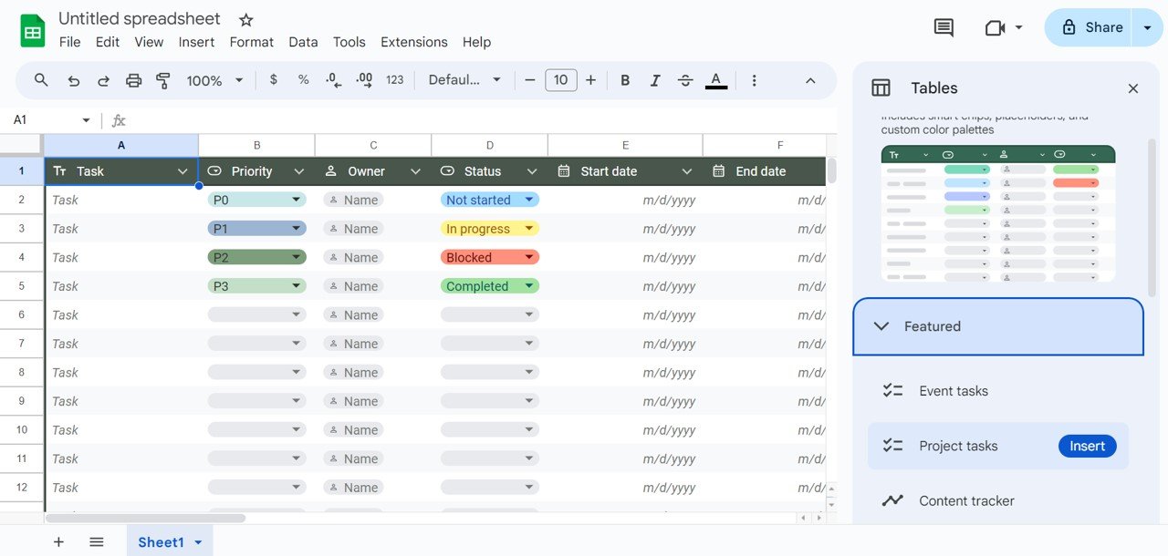
Note: If Templates pane is not available by default then you can Right click anywhere on the sheet and click on Tables.
Data Type of Columns:
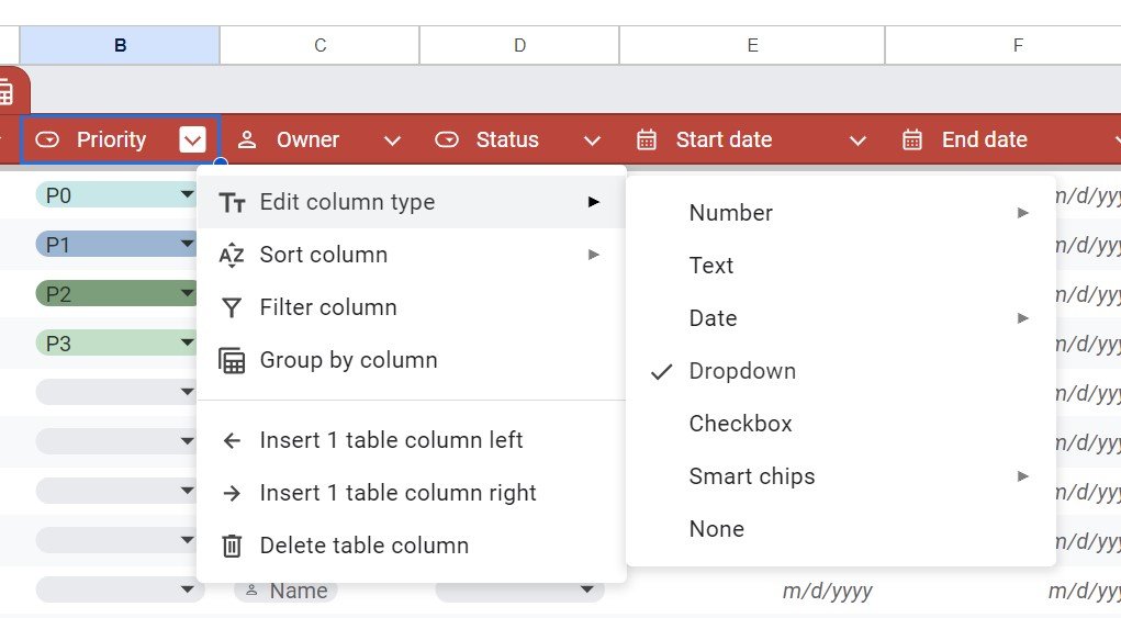
In the table, you can change the data type in the table of columns by following the below steps:
- Go to the down arrow icon in front of the column name.
- Go to the Edit Column Type.
- Now, you can select the data type as Number, Text, Date, Drop down, Check box etc.
Convert normal into a Table:
To convert your normal data range into a table format, follow the below given instructions:
- Select the range.
- Go to the format and Click on Convert To Table.
- Alternatively, you can right-click and click on Tables.
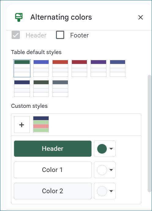
Change the Table Formatting:
If you want to change the table formatting like header colors for alternative rows color then follow the below steps:
- Click any where on the table.
- Go to the Format and click on the Alternating Colors.
- Alternating Colors pane will be opened.
- Choose the default table layout or create the custom one.
Group By Column:
You can Group the data by any column by following the below steps:
- Click on the down arrow icon in front of the column name.
- Click on the Group by the column.
- Table will be grouped by that table.
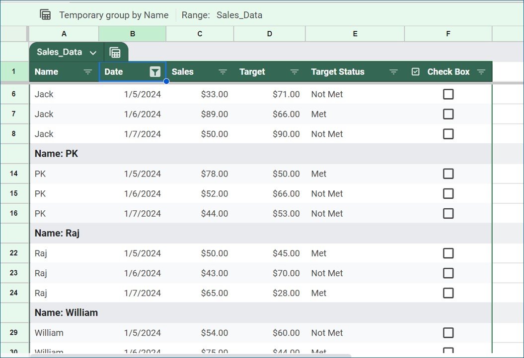
You can save this group as a view using the Save View button available on the Top right corner of the sheet.
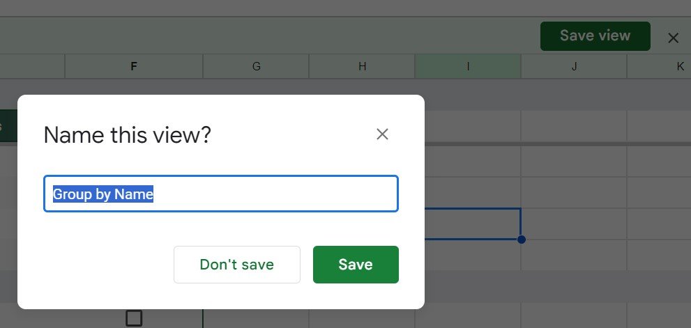
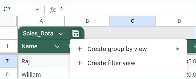
Filter View:
You can save a filter view also by using the View button and click on the Create Filter View. Just follow the below steps:
- Now you can put the filters on any column or sort the data.
- Click on the Save view button and give a name.
Now this view will be available with that name to see again quickly.
Rename the table:
You can rename the table with just a click on the default table name on the top right corner of the table and put the name which you want to put.
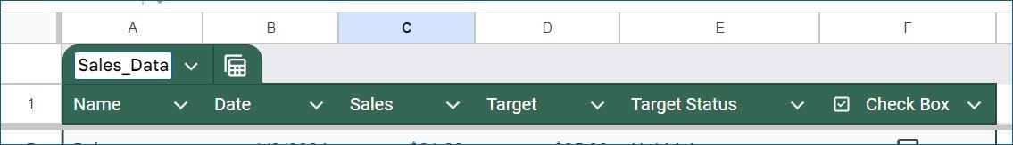
Using the formula with table:
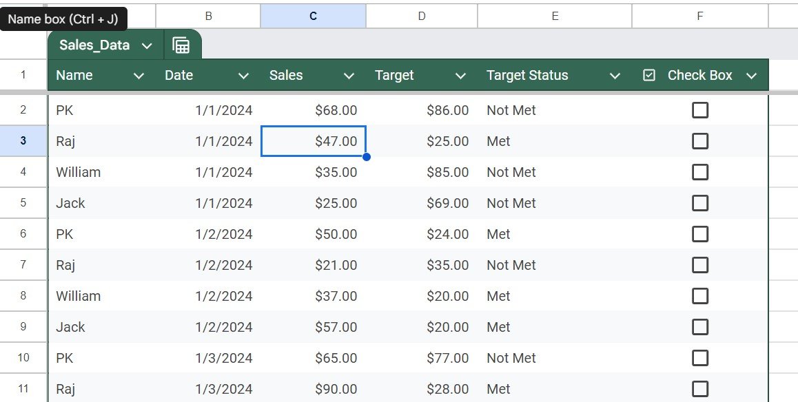
Using the formula with the table is quite easy. You can refer the table name and field name in the table as given in below example:
=SUM(Sales_Data[Sales])
Visit our YouTube channel to learn step-by-step video tutorials
Youtube.com/@NeotechNavigators

