If you still reach for VLOOKUP every time you need to pull a value from another sheet, this tutorial will change how you work. XLOOKUP in Google Sheets is now available, and it fixes almost every complaint people ever had about VLOOKUP: it looks left, it handles missing values on its own, it returns several columns at once, and it can search a list from the bottom up.
In this step-by-step guide we will build five real formulas in a practice file, plus one bonus two-way lookup. Every screenshot below is taken from the finished file, so you can compare your result with mine at each step.
Free practice file: open the XLOOKUP practice sheet and use File → Make a copy so you can type along.
Syntax: XLOOKUP in Google Sheets
XLOOKUP takes six arguments, and only the first three are required:
=XLOOKUP(search_key, lookup_range, result_range, [missing_value], [match_mode], [search_mode])| Argument | Required? | What it does |
|---|---|---|
search_key |
Yes | The value you are looking for |
lookup_range |
Yes | The single column (or row) to search in |
result_range |
Yes | What to return — can be several columns wide |
missing_value |
No | What to show when nothing matches, instead of #N/A |
match_mode |
No | 0 exact (default), -1 next smaller, 1 next larger, 2 wildcard |
search_mode |
No | 1 top to bottom (default), -1 bottom to top |
The two things to notice straight away: the lookup range and the result range are separate arguments — there is no column index number to count, and no rule that says the answer must sit to the right of the key.
The practice data
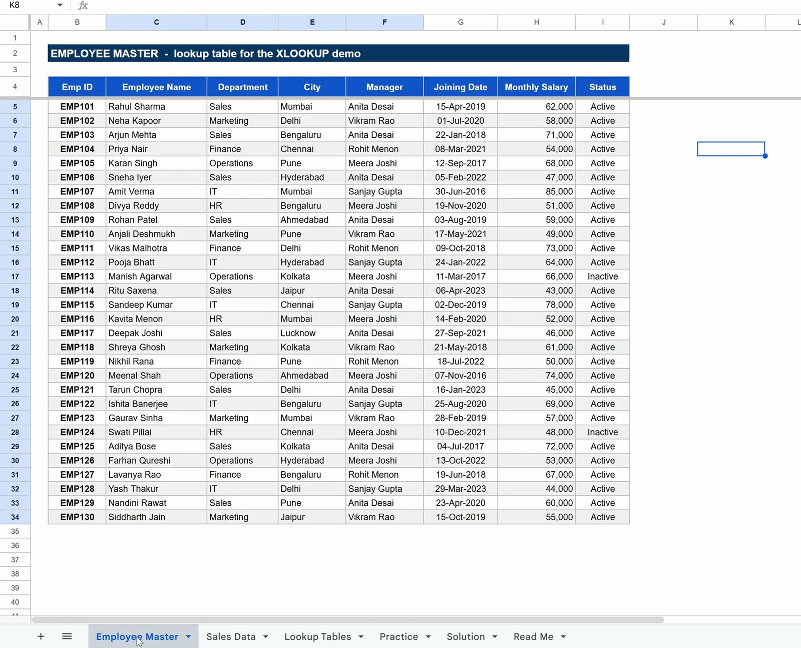
The practice file has three data sheets. The main one is Employee Master — 30 employees with Emp ID, Employee Name, Department, City, Manager, Joining Date, Monthly Salary and Status.
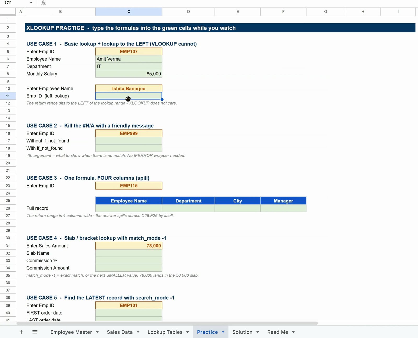
The Practice sheet is where you will work. The yellow cells are the inputs, already filled in, and the green cells are empty — that is where each formula goes.
Use Case 1 — Basic lookup, and a lookup to the LEFT
Step 1: Pull the employee name
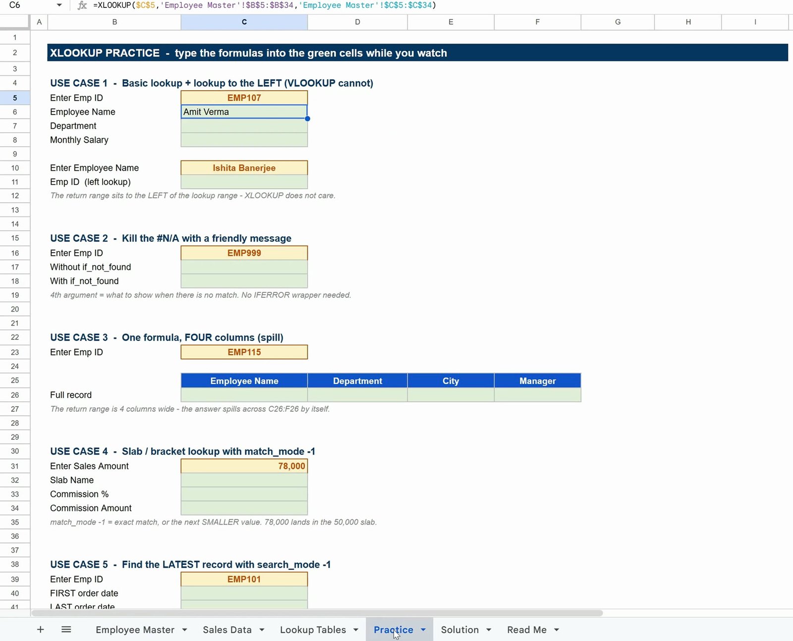
Cell C5 holds the Emp ID we are searching for (EMP107). Click cell C6 and type:
=XLOOKUP($C$5,'Employee Master'!$B$5:$B$34,'Employee Master'!$C$5:$C$34)Read it out loud and it makes sense: search for the value in C5, inside column B of Employee Master, and give me the matching value from column C.
Step 2: Reuse the formula for Department and Salary
Do not type the whole thing again. Copy the finished formula out of the formula bar, paste it into C7, and change only the result range:
=XLOOKUP($C$5,'Employee Master'!$B$5:$B$34,'Employee Master'!$D$5:$D$34)   ← Department
=XLOOKUP($C$5,'Employee Master'!$B$5:$B$34,'Employee Master'!$H$5:$H$34)   ← Monthly Salary
Because the ranges are locked with $ signs, only one piece ever changes.
Step 3: The lookup VLOOKUP cannot do
Now flip the question around. Cell C10 holds an employee name, and we want the Emp ID — which sits in the column to the left of the name. VLOOKUP simply cannot do this without INDEX + MATCH. XLOOKUP does not care:
=XLOOKUP($C$10,'Employee Master'!$C$5:$C$34,'Employee Master'!$B$5:$B$34)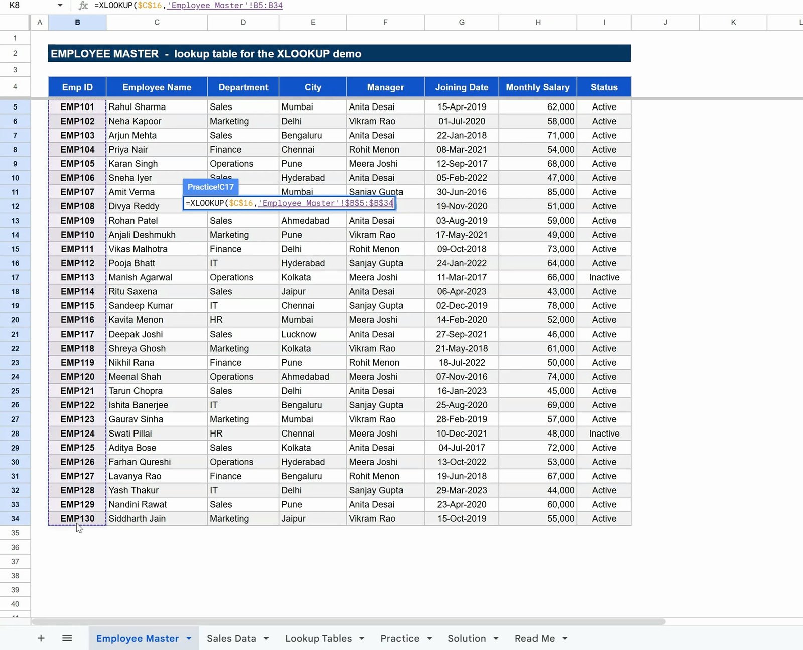
Swap the two ranges and the direction of the lookup changes. That is the whole trick.
Use Case 2 — Kill #N/A with a friendly message
Type an Emp ID that does not exist, such as EMP999, and a plain XLOOKUP returns #N/A:
=XLOOKUP($C$16,'Employee Master'!$B$5:$B$34,'Employee Master'!$C$5:$C$34)You do not need an IFERROR wrapper. The fourth argument is built for exactly this:
=XLOOKUP($C$16,'Employee Master'!$B$5:$B$34,'Employee Master'!$C$5:$C$34,"Employee Not Found")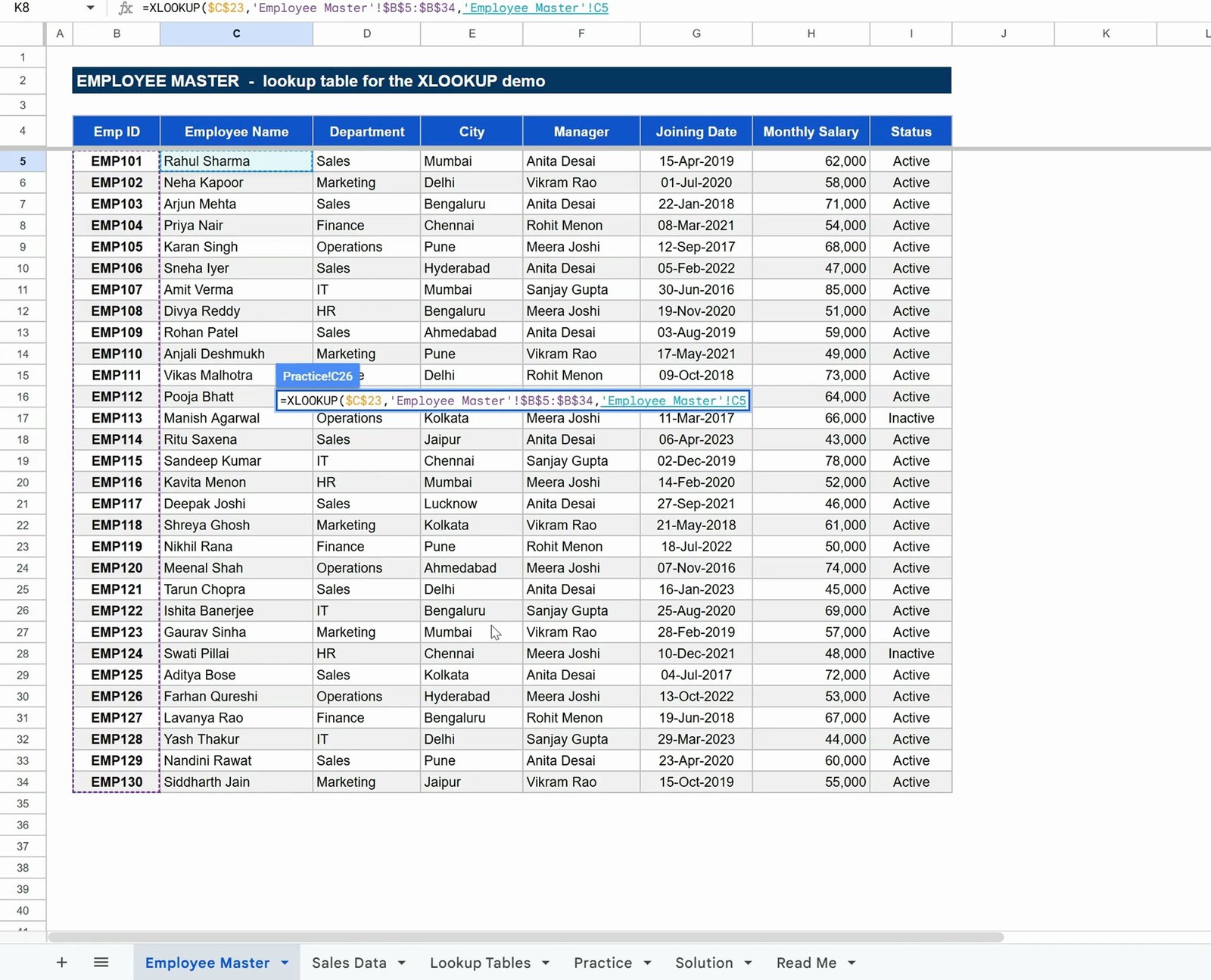
This is also safer than IFERROR. IFERROR hides every error — including a broken reference or a typo in your range. missing_value only handles “no match found”, so a real mistake still shows up.
Use Case 3 — One formula, four columns
Here is where most people stop thinking of XLOOKUP as “a better VLOOKUP”. The result range does not have to be one column wide. Make it four columns, and one formula fills four cells:
=XLOOKUP($C$23,'Employee Master'!$B$5:$B$34,'Employee Master'!$C$5:$F$34,"Not Found")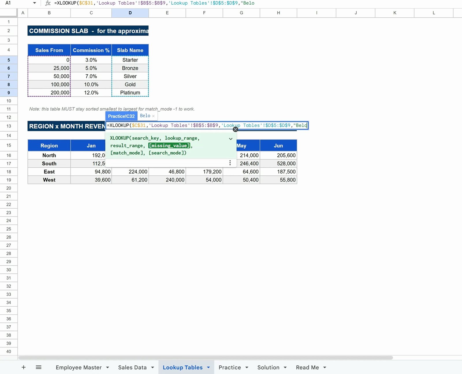
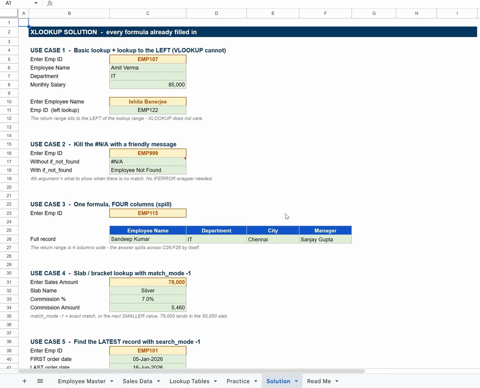
Type it in C26 and the answer spills across C26:F26 — Employee Name, Department, City and Manager, all from a single formula. No dragging, no four separate lookups to keep in sync.
Tip: leave the cells to the right empty. If anything is sitting in them the formula returns a spill error instead.
Use Case 4 — Slab and bracket lookup with match_mode -1
This is the commission-slab problem, and it is where the fifth argument earns its keep. The Lookup Tables sheet holds the slabs:
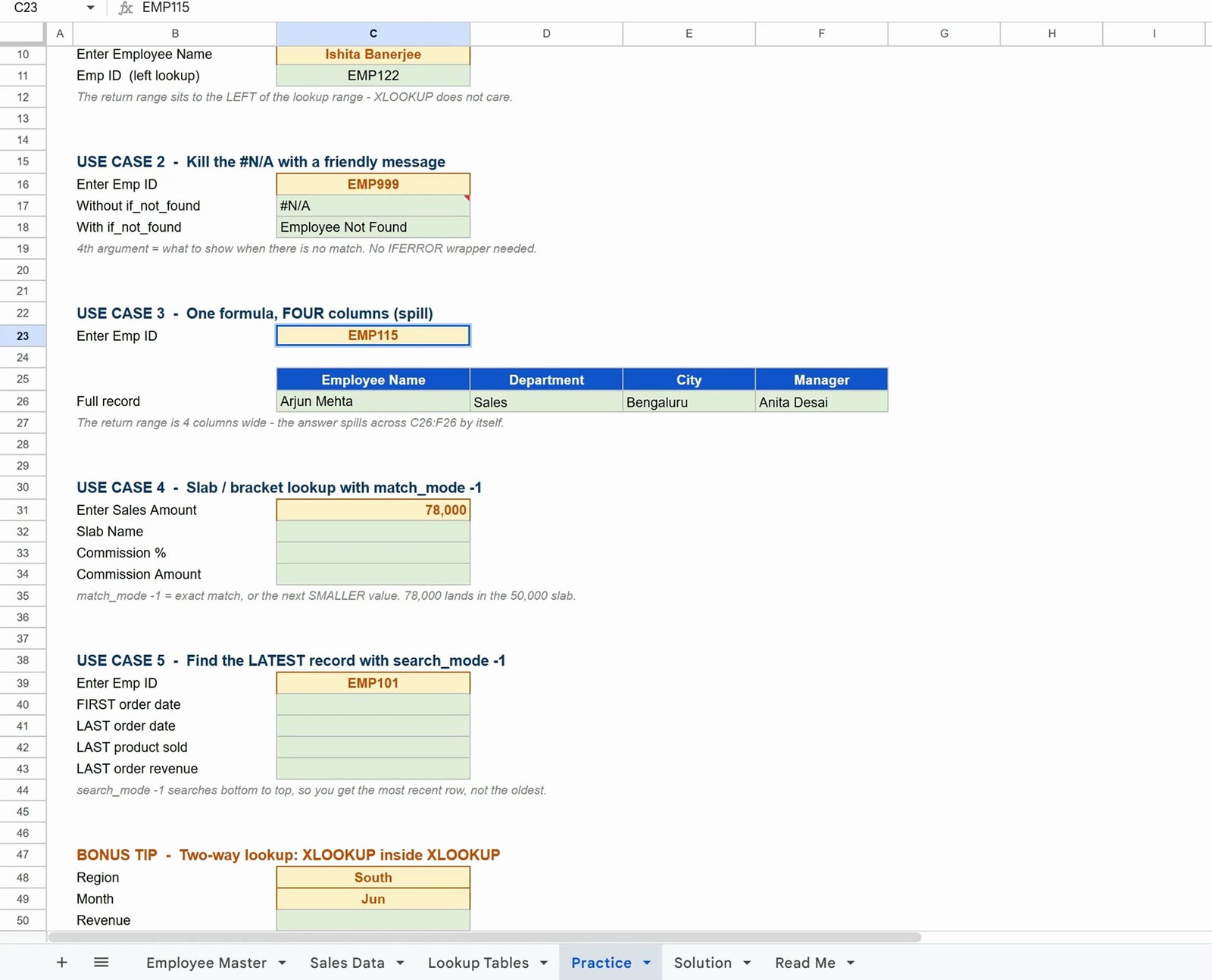
The sales amount we are looking up is 78,000 — a number that appears nowhere in the table. It falls between 50,000 and 100,000, so we want the 50,000 row. That is what match_mode -1 means: if there is no exact match, take the next smaller value.
=XLOOKUP($C$31,'Lookup Tables'!$B$5:$B$9,'Lookup Tables'!$D$5:$D$9,"Below slab",-1)   ← Slab Name
=XLOOKUP($C$31,'Lookup Tables'!$B$5:$B$9,'Lookup Tables'!$C$5:$C$9,0,-1)              ← Commission %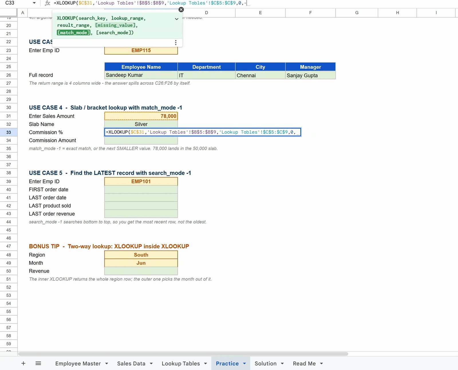
78,000 lands in the 50,000 slab: Silver, 7.0%, giving a commission of 5,460. Change the sales amount and the slab follows automatically.
One rule you must not forget: the slab table has to be sorted from smallest to largest for match_mode -1 to work.
Use Case 5 — Find the LATEST record with search_mode -1
The Sales Data sheet lists 50 orders, sorted oldest first. One employee can appear many times.
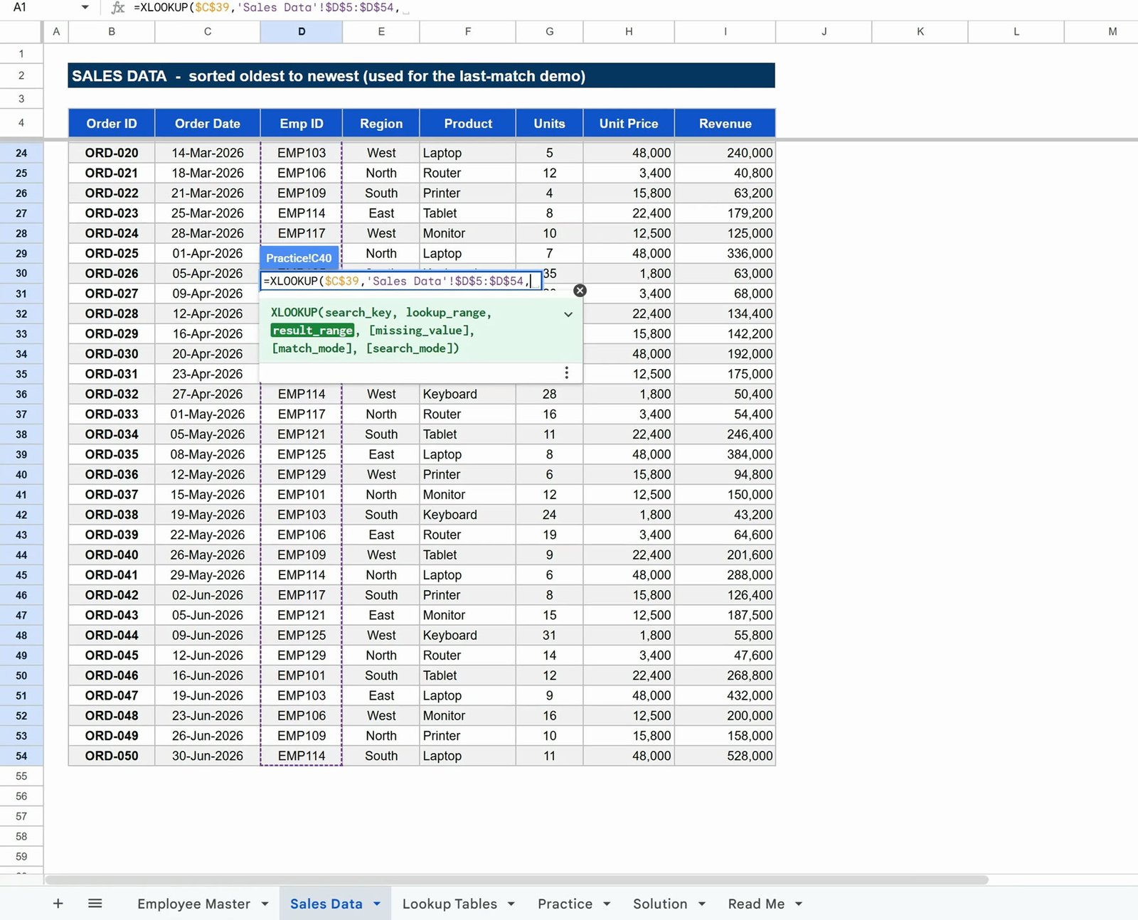
A normal XLOOKUP searches top to bottom, so it returns the employee’s first order:
=XLOOKUP($C$39,'Sales Data'!$D$5:$D$54,'Sales Data'!$C$5:$C$54,"None")Set the sixth argument to -1 and the search runs bottom to top, which gives you the most recent row instead:
=XLOOKUP($C$39,'Sales Data'!$D$5:$D$54,'Sales Data'!$C$5:$C$54,"None",0,-1)   ← LAST order date
=XLOOKUP($C$39,'Sales Data'!$D$5:$D$54,'Sales Data'!$F$5:$F$54,"None",0,-1)   ← LAST product sold
=XLOOKUP($C$39,'Sales Data'!$D$5:$D$54,'Sales Data'!$I$5:$I$54,0,0,-1)        ← LAST order revenue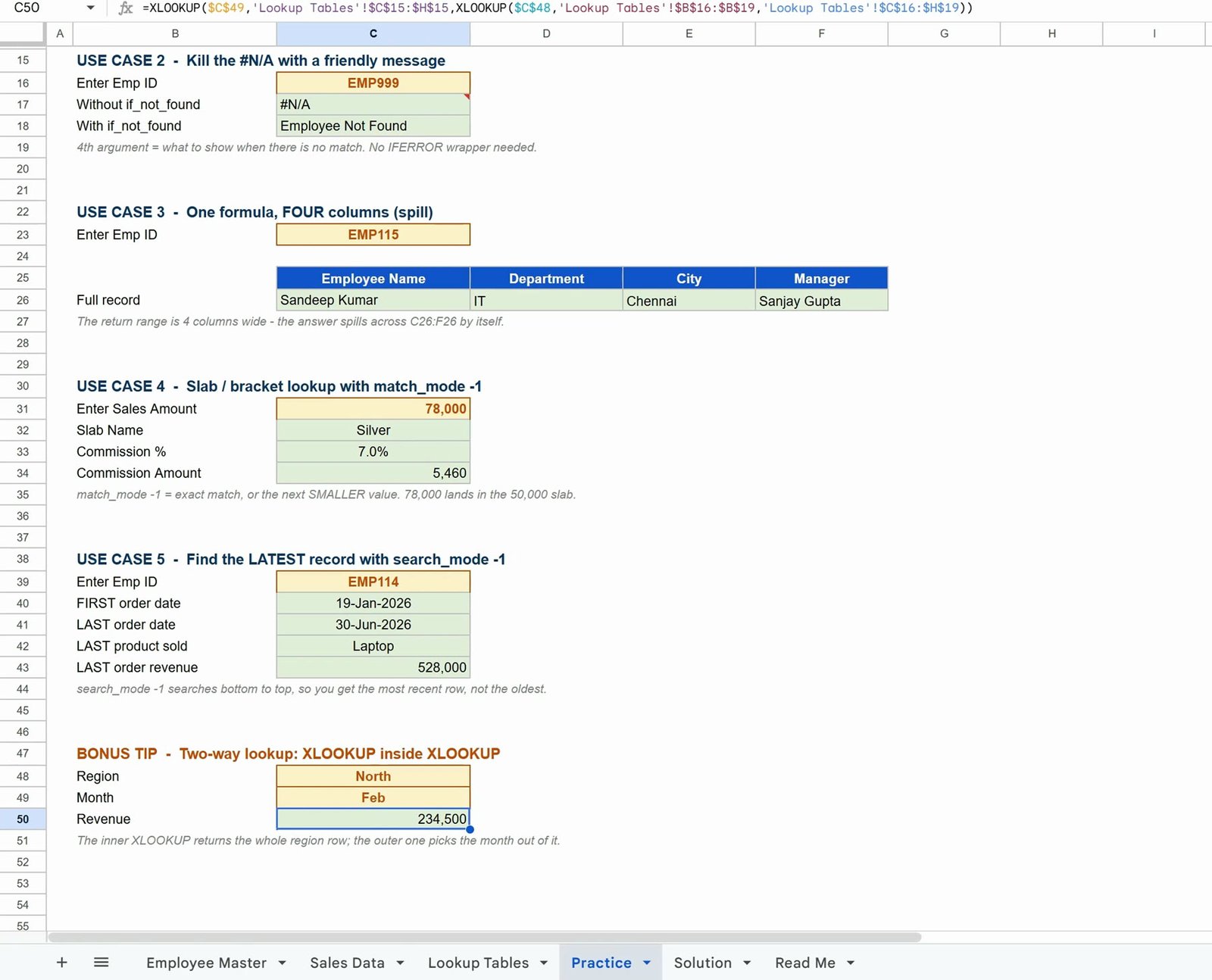
Notice the 0 in the fifth position — you still have to pass match_mode (exact) before you can reach search_mode. This one argument replaces the MAXIFS-and-INDEX gymnastics most people use for “latest record” reports.
Bonus tip — A two-way lookup: XLOOKUP inside XLOOKUP
The last table on the Lookup Tables sheet is a revenue grid: regions down the side, months across the top. We want the value where a region and a month meet.
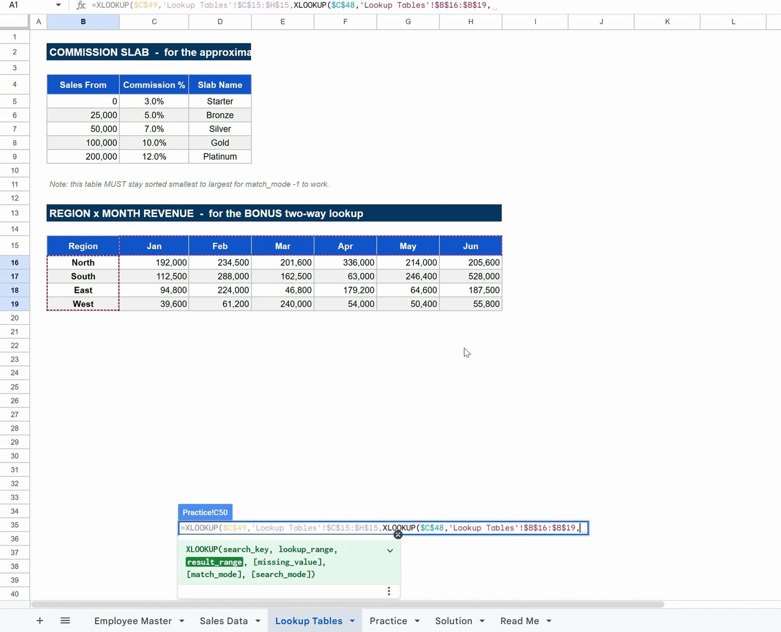
Put one XLOOKUP inside another. The inner one picks the whole row for the region; the outer one picks the month out of that row:
=XLOOKUP($C$49,'Lookup Tables'!$C$15:$H$15,XLOOKUP($C$48,'Lookup Tables'!$B$16:$B$19,'Lookup Tables'!$C$16:$H$19))Region South and month Jun returns 528,000. Change either input and the answer updates — a full matrix lookup in one formula, no INDEX, no MATCH, no helper column.
The finished sheet
The practice file also has a Solution sheet with every formula already filled in, so you can check your work:
XLOOKUP formula cheat sheet
| You want to… | Formula pattern |
|---|---|
| Basic lookup | =XLOOKUP(key, lookup_col, result_col) |
| Look to the left | Swap the lookup and result ranges — nothing else changes |
Replace #N/A |
=XLOOKUP(key, lookup_col, result_col, "Not Found") |
| Return several columns | Make result_range multiple columns wide |
| Slab / bracket lookup | =XLOOKUP(key, slab_col, result_col, "Below slab", -1) |
| Latest matching record | =XLOOKUP(key, lookup_col, result_col, "None", 0, -1) |
| Two-way (row × column) | =XLOOKUP(col_key, header_row, XLOOKUP(row_key, row_labels, grid)) |
Frequently asked questions
Is XLOOKUP available in Google Sheets?
Yes. XLOOKUP rolled out to Google Sheets and works in any normal Google account — there is nothing to install or enable.
Is XLOOKUP better than VLOOKUP in Google Sheets?
For almost every real job, yes. It looks left as easily as right, it needs no column index number, it handles missing values without IFERROR, it can return several columns at once, and it can search a list from the bottom up. VLOOKUP does none of these.
Do I still need INDEX and MATCH?
Much less often. The two classic reasons for INDEX + MATCH — looking to the left and two-way lookups — are both covered here, the second one by nesting XLOOKUP inside itself.
Why does my XLOOKUP return a spill error?
Because the result range is more than one column wide and something is already sitting in the cells the answer needs. Clear those cells and the formula spills correctly.
Why does my slab lookup return the wrong band?
Almost always because the slab table is not sorted smallest to largest. match_mode -1 assumes an ascending list.
Watch the full tutorial
Every formula above is built on screen, step by step, in the video version of this tutorial on the NeoTech Navigators YouTube channel. Grab the free practice file, make a copy, and type along — that is the fastest way to make these stick.
For more Google Sheets formulas, dashboards and ready-made templates, visit NeoTechNavigators.com.
Download the free practice file
Everything you need in one page: the view-only Google Sheets link, a one-click Make a copy link, and the full formula cheat sheet from this tutorial.
Free · No sign-up · Opens the Google Sheet in view-only mode, then copy it to your own Drive