You download a customer list from some software, open it in Google Sheets, and it is a mess. Names have extra spaces. Some are in capitals, some in small letters. A few email addresses are broken, and the same order appears three times. Before you can build a report from that data, you have to clean it, and doing it by hand can take hours.
In this step-by-step tutorial you will clean all of it in seconds with five simple Google Sheets tricks (TRIM and CLEAN, PROPER/LOWER/UPPER, SPLIT, UNIQUE and ISEMAIL) plus a bonus trick that cleans a whole column with one formula. Every screenshot below comes from the finished practice file, so you can check your result at each step.
Free practice file: make your own copy of the practice sheet and type along. The download at the end of this post has the view link, the copy link and the full formula cheat sheet.
Watch the video tutorial
Video overview
The 11-minute video builds every formula on screen, slowly and one step at a time. It starts with a practice sheet full of messy data: names with hidden spaces, a name split over two lines by a line break, names and emails in random capitals, “City, State” in one cell, an order list with three repeated orders, and eight email addresses of which four are broken. Tip by tip, the green cells fill in: TRIM and CLEAN remove the spaces and invisible characters, PROPER, LOWER and UPPER fix the capitals, SPLIT separates names and places, UNIQUE and the Remove duplicates menu take 12 orders down to 9, and ISEMAIL flags the four bad addresses. The bonus shows how ARRAYFORMULA runs TRIM and PROPER on a whole column from a single cell. The chapters are listed below the video on YouTube.
What you will learn
- TRIM + CLEAN: remove extra spaces and hidden line breaks
- PROPER, LOWER and UPPER: fix capital letters in names, emails and codes
- SPLIT and Data > Split text to columns: break one column into many
- UNIQUE and Data > Data cleanup > Remove duplicates: drop repeated rows
- ISEMAIL: catch broken email addresses before you send anything
- Bonus: ARRAYFORMULA: clean a whole column with one formula
The practice file
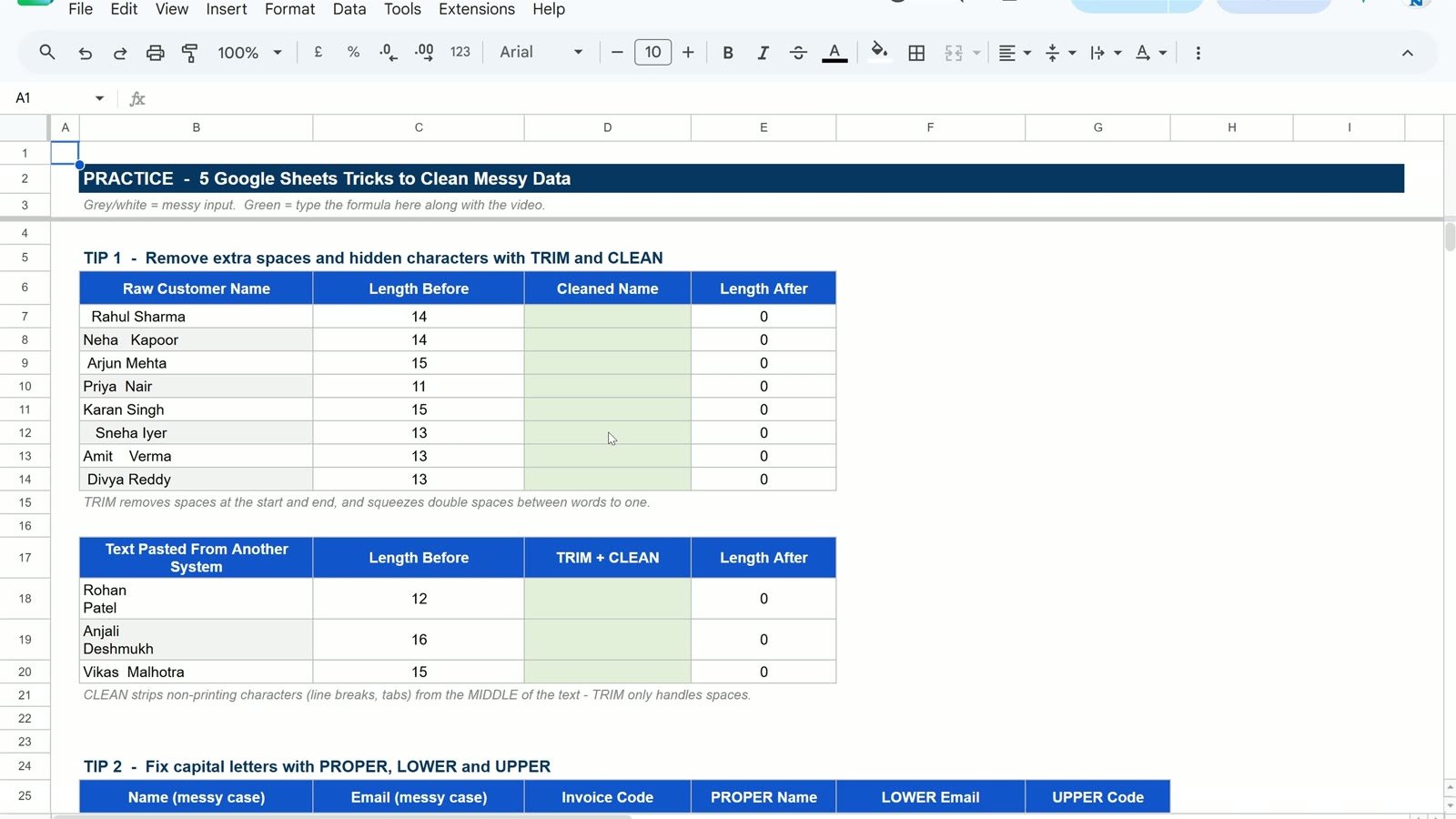
The file has three sheets. Practice is where you work, Solution has every formula already written, and Read Me explains each tip. On the Practice sheet the white and grey cells hold the messy data and the green cells are empty. That is where you type the formulas.
Tip 1: Remove extra spaces and hidden characters with TRIM and CLEAN
Look at the first table. “Rahul Sharma” has two spaces in front of the name, and “Neha Kapoor” has three spaces in the middle. Some spaces you can see and some you cannot, which is why the practice file has a Length Before column (=LEN(B7)). It counts every character, including spaces: “Rahul Sharma” is only 12 characters, but the length says 14.
Step 1: Type the TRIM formula
Click cell D7 and type:
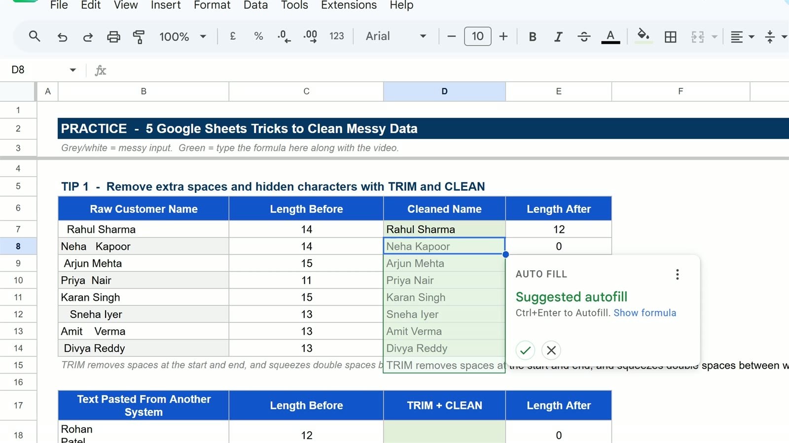
=TRIM(B7)Press Enter. The result is Rahul Sharma, and the Length After column drops from 14 to 12: both extra spaces are gone. Google Sheets may also offer a Suggested autofill for the rest of the column.
Step 2: Copy it down
Click D7, press Ctrl + C, select D8:D14 and press Ctrl + V. Look at Neha Kapoor: the three spaces in the middle have become one. TRIM removes spaces at the start, spaces at the end, and squeezes repeated spaces between words down to one.
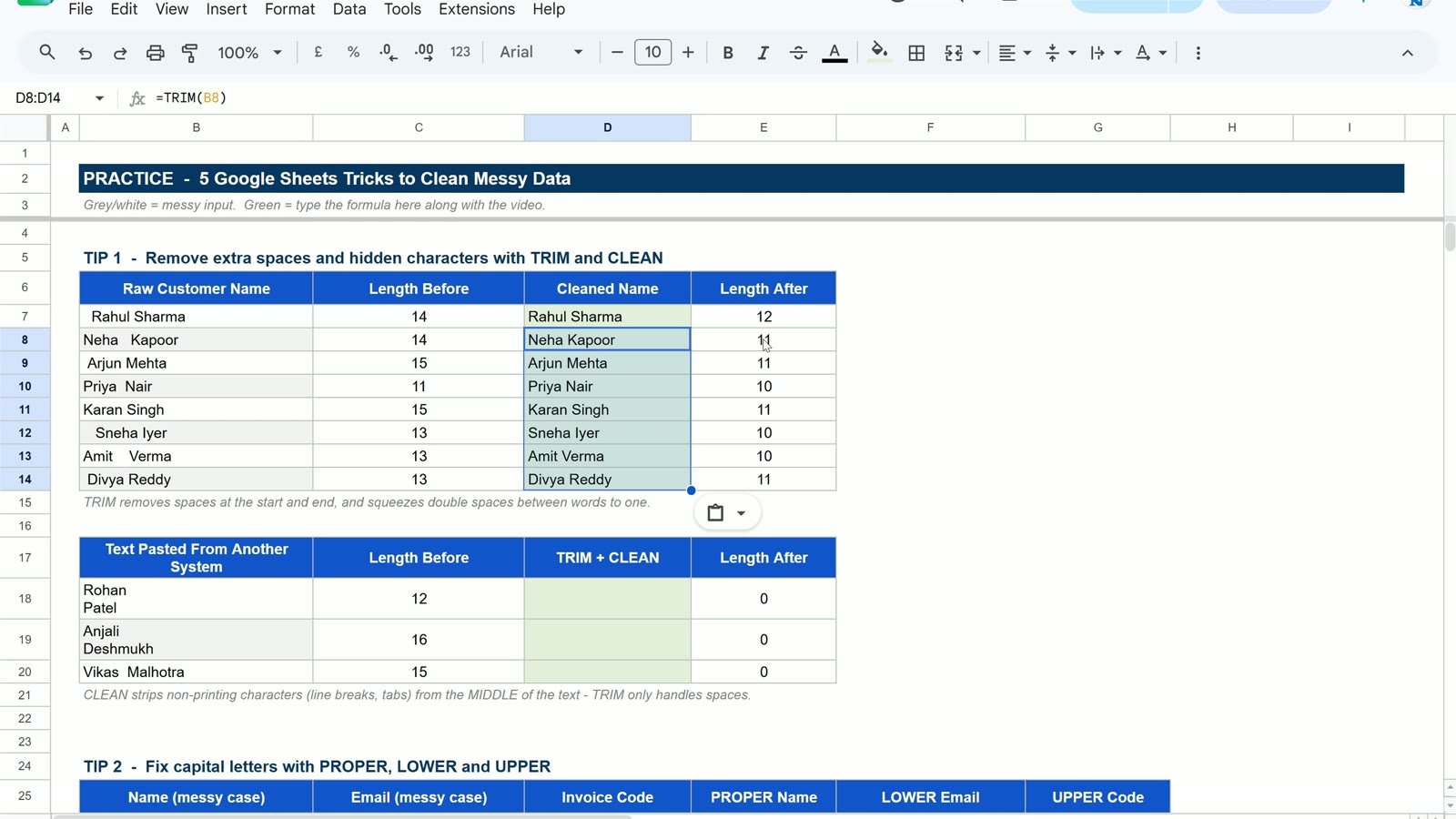
Step 3: Add CLEAN for line breaks and tabs
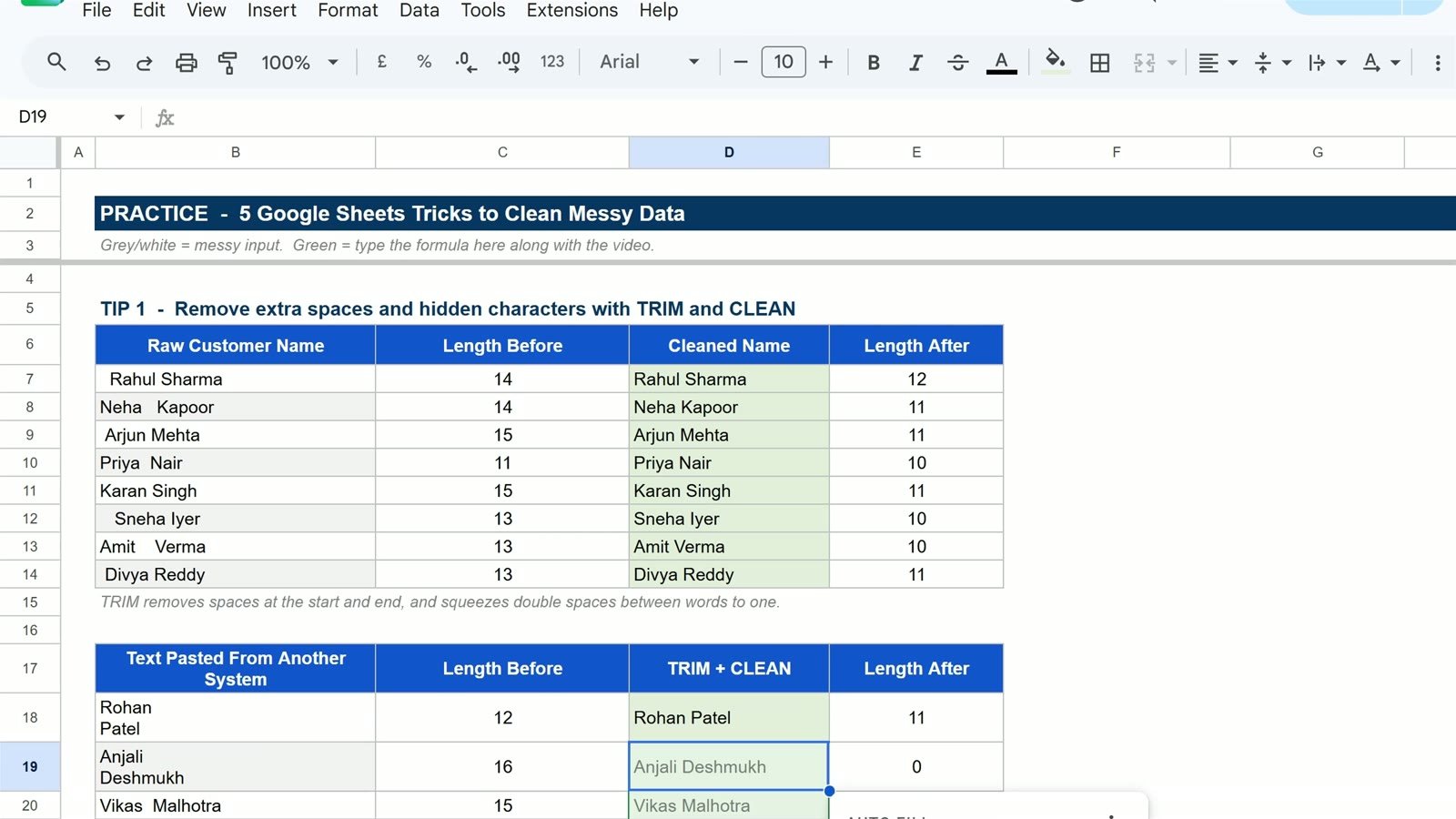
The second table holds text pasted from another system. “Rohan Patel” shows on two lines because a line break sits in the middle of the name, and TRIM cannot remove it: TRIM only handles spaces. Wrap CLEAN inside TRIM. In D18 type:
=TRIM(CLEAN(B18))Rohan Patel is back on one line and the length goes from 12 to 11. Copy it to D19:D20: “Vikas Malhotra” had a hidden tab character, and that is gone too. Rule of thumb: TRIM for spaces, CLEAN for invisible characters, and use them together.
Tip 2: Fix capital letters with PROPER, LOWER and UPPER
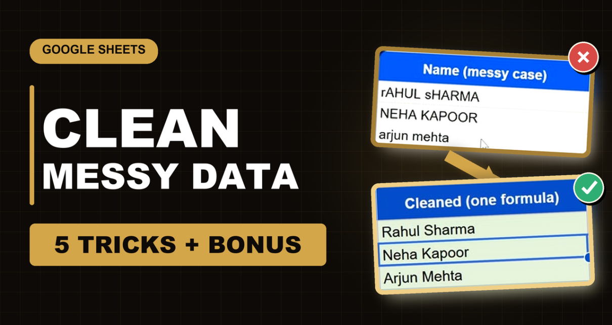
In this table the names are typed every possible way (rAHUL sHARMA, NEHA KAPOOR, arjun mehta), the emails are in mixed case and the invoice codes are mixed too.
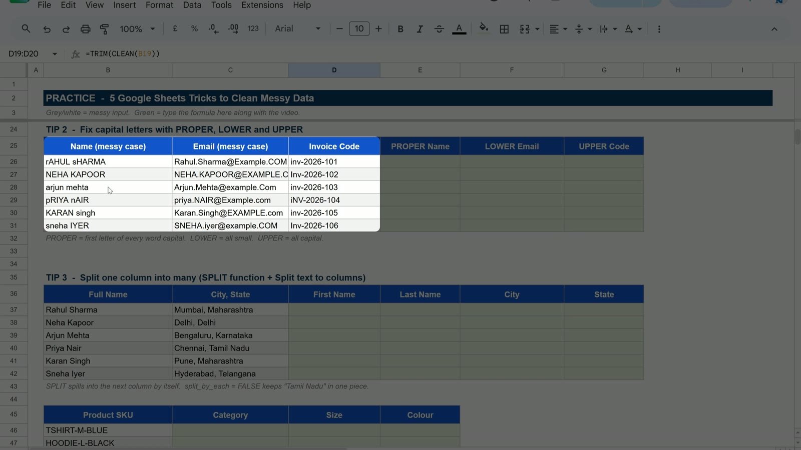
Google Sheets has one function for each job. Type these three formulas in row 26:
E26:  =PROPER(B26)   → Rahul Sharma (first letter of every word capital)
F26:  =LOWER(C26)    → rahul.sharma@example.com (all small letters)
G26:  =UPPER(D26)    → INV-2026-101 (all capitals)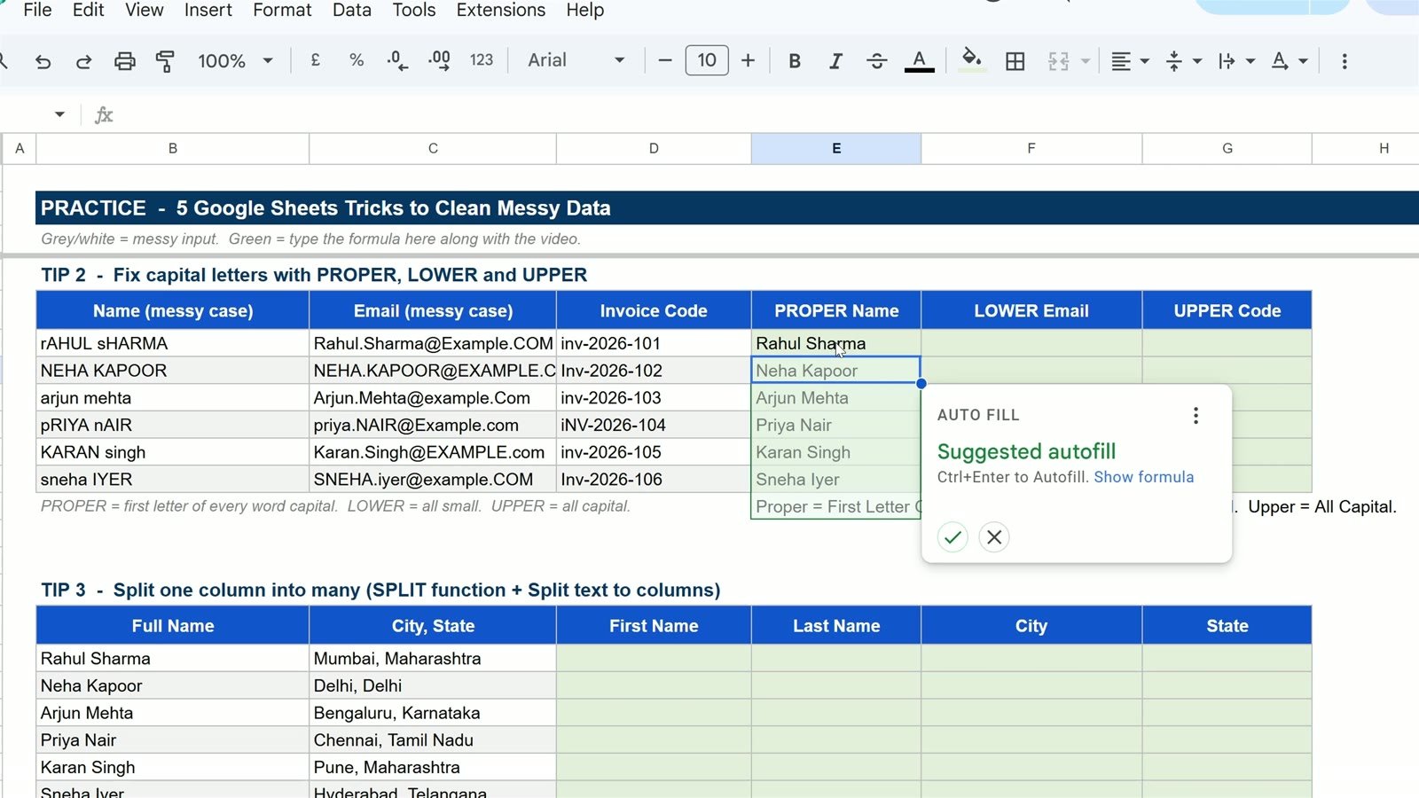
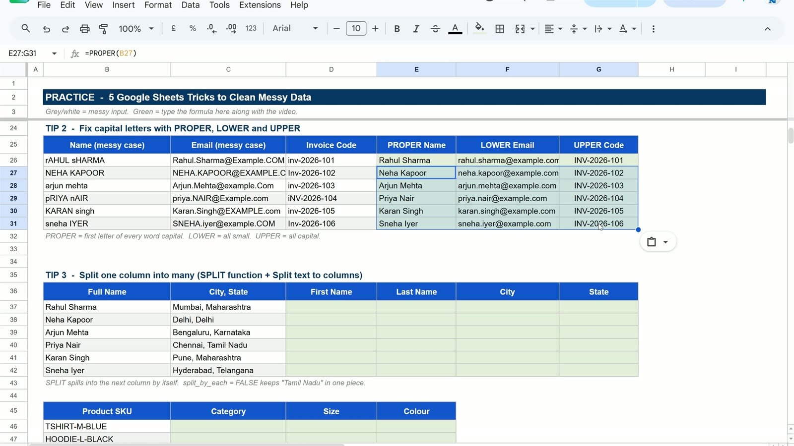
Then select E26:G26, copy, select E27:G31 and paste. All six rows are cleaned in one go.
Tip 3: Split one column into many
The SPLIT function
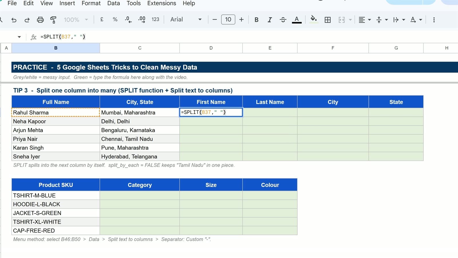
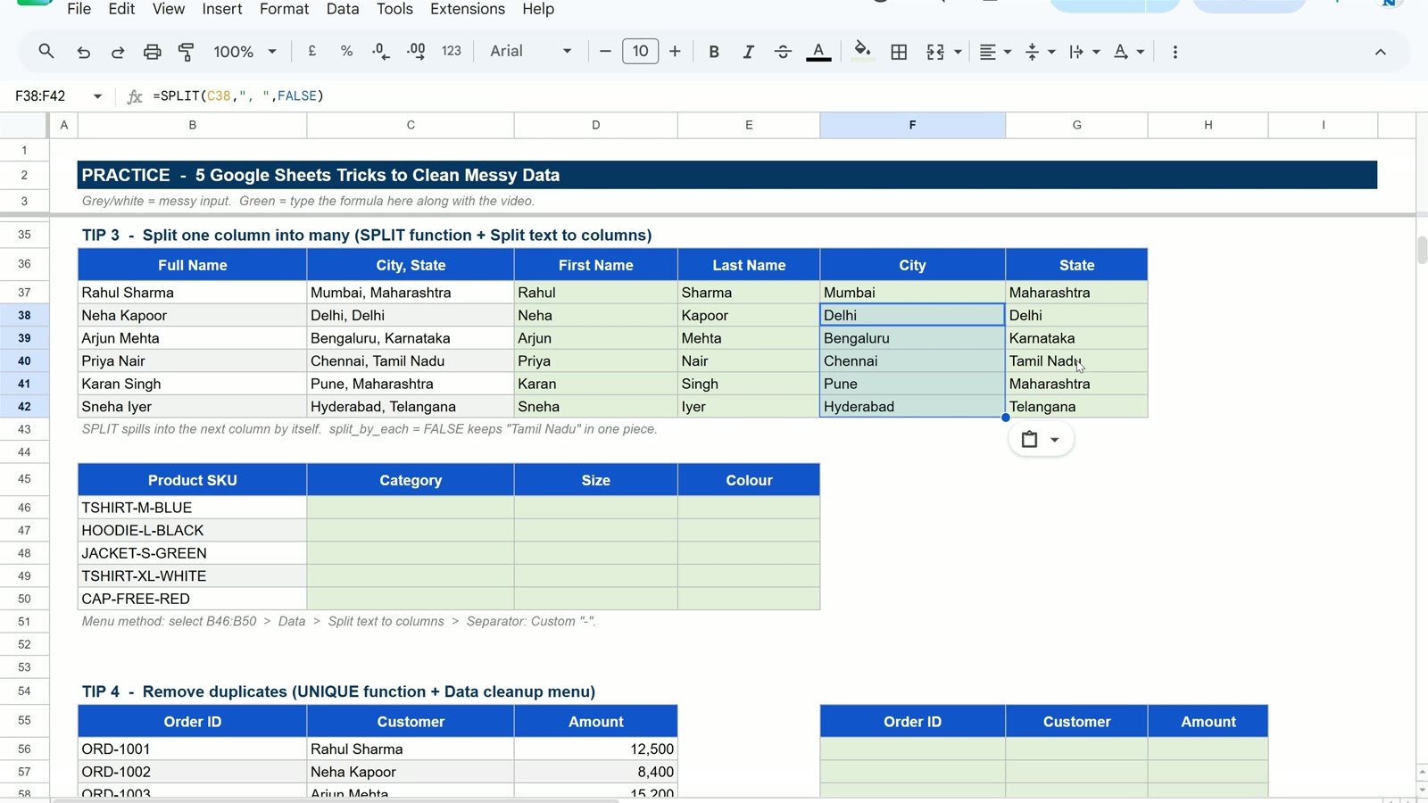
The full name sits in one cell, but you want first and last name in separate columns. In D37 type:
=SPLIT(B37," ")The space in the quotes is the separator. “Rahul” lands in column D and “Sharma” spills into column E by itself, although you typed the formula in one cell only.
For “City, State” use a comma and a space as the separator, and add FALSE:
=SPLIT(C37,", ",FALSE)That third argument (split_by_each) set to FALSE tells Google Sheets to treat “, ” as one separator. Without it, every comma and every space would split the text, and “Tamil Nadu” would break into two pieces.
The menu way: Split text to columns
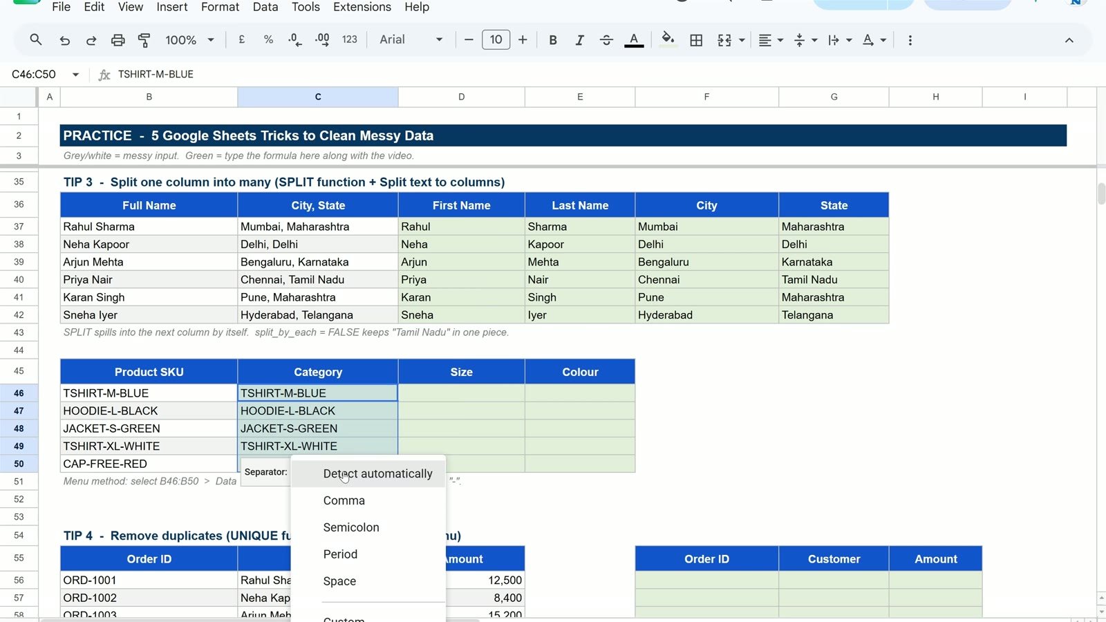
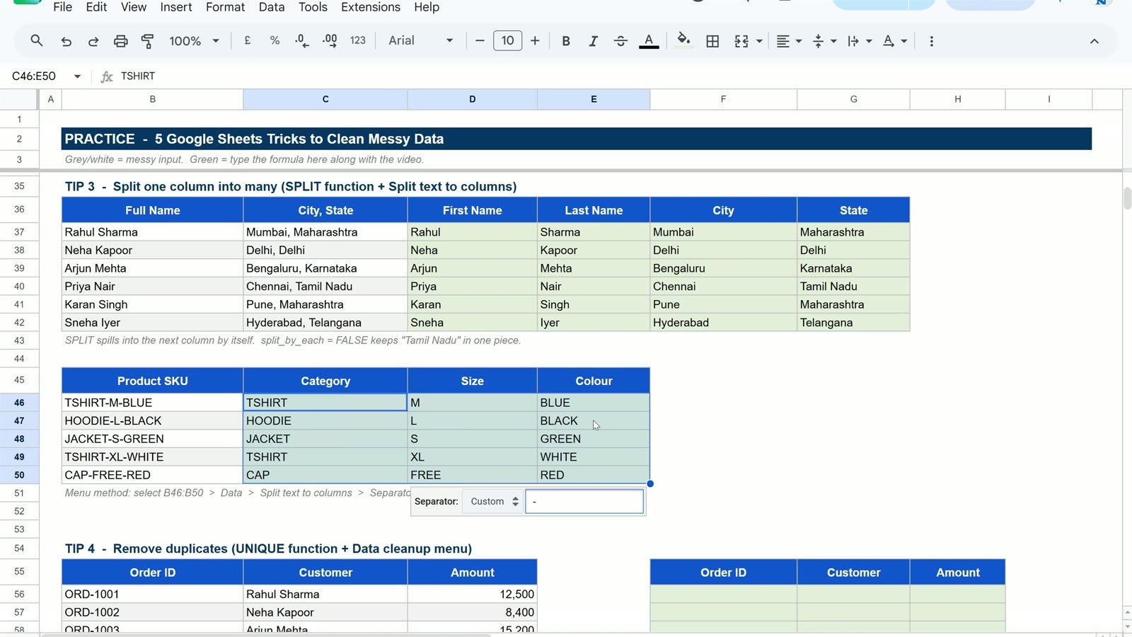
Below, the product codes join the category, size and colour with a dash (TSHIRT-M-BLUE). First copy the codes into the Category column (Ctrl + Shift + V pastes values only), so the originals stay safe. Then go to Data > Split text to columns, open the separator list and choose Custom, then type a dash.
Tip 4: Remove duplicates with UNIQUE and Data cleanup
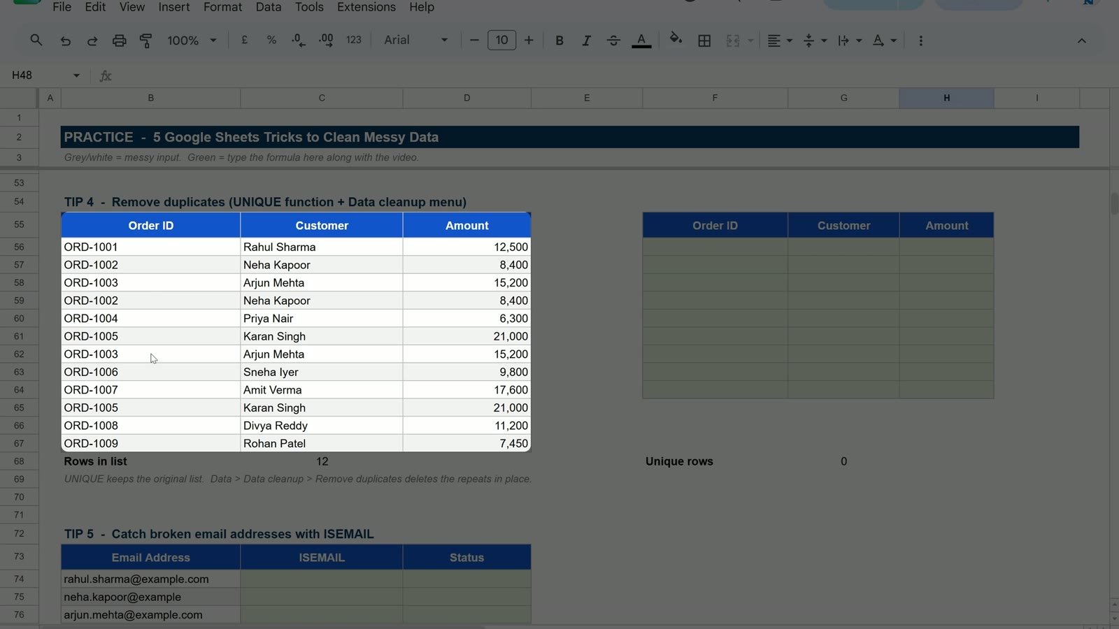
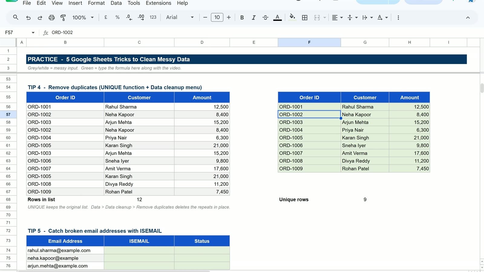
This order list has 12 rows, but ORD-1002, ORD-1003 and ORD-1005 each appear twice. Total this list and your sales figure will be wrong.
The formula way: UNIQUE
In F56 type the formula below and select the whole list, B56 to D67:
=UNIQUE(B56:D67)You get 9 unique orders, and the original list is not touched at all. The counters under the tables show 12 rows in the list and 9 unique rows.
The menu way: Remove duplicates
To delete the repeats from the list itself, select B56:D67 and go to Data > Data cleanup > Remove duplicates. The same submenu also has Trim whitespace, which trims a whole range without a formula.
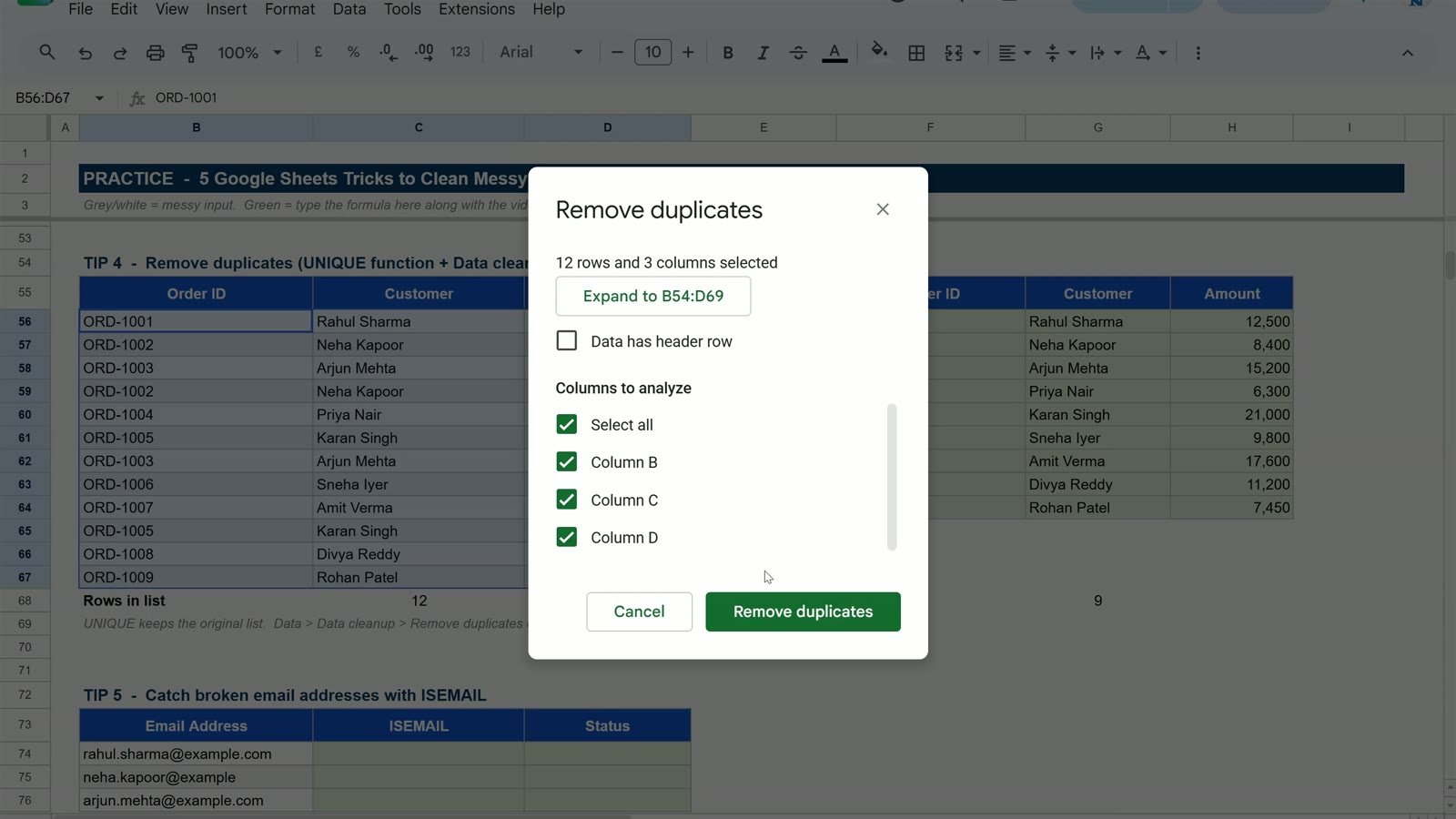
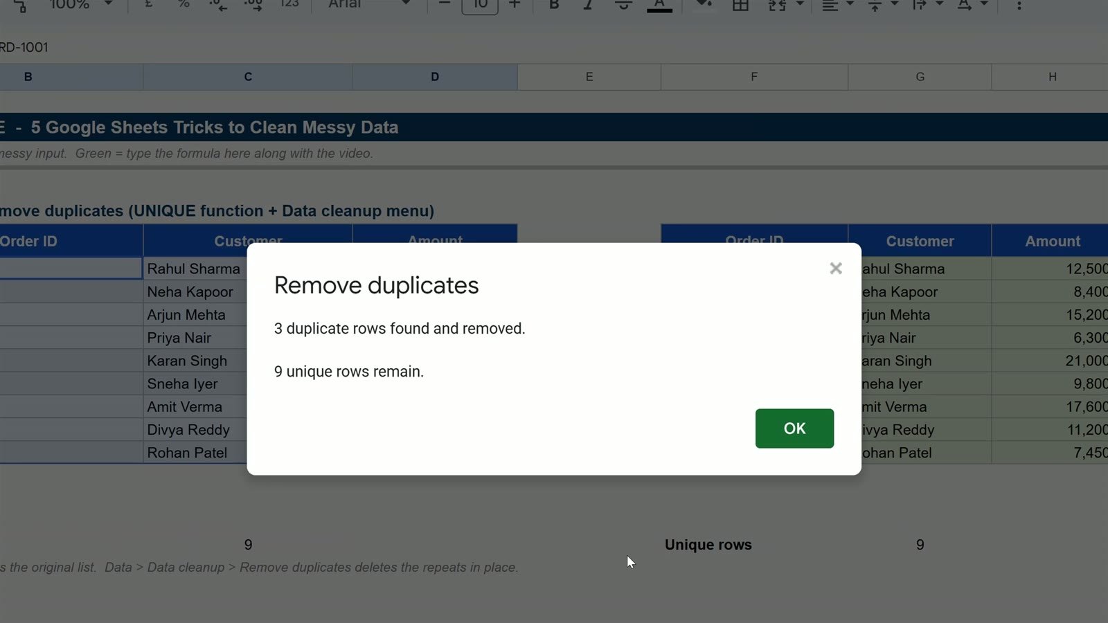
Click the Remove duplicates button. Google Sheets reports “3 duplicate rows found and removed. 9 unique rows remain.” Click OK, and the count under the list changes from 12 to 9.
Tip 5: Catch broken email addresses with ISEMAIL
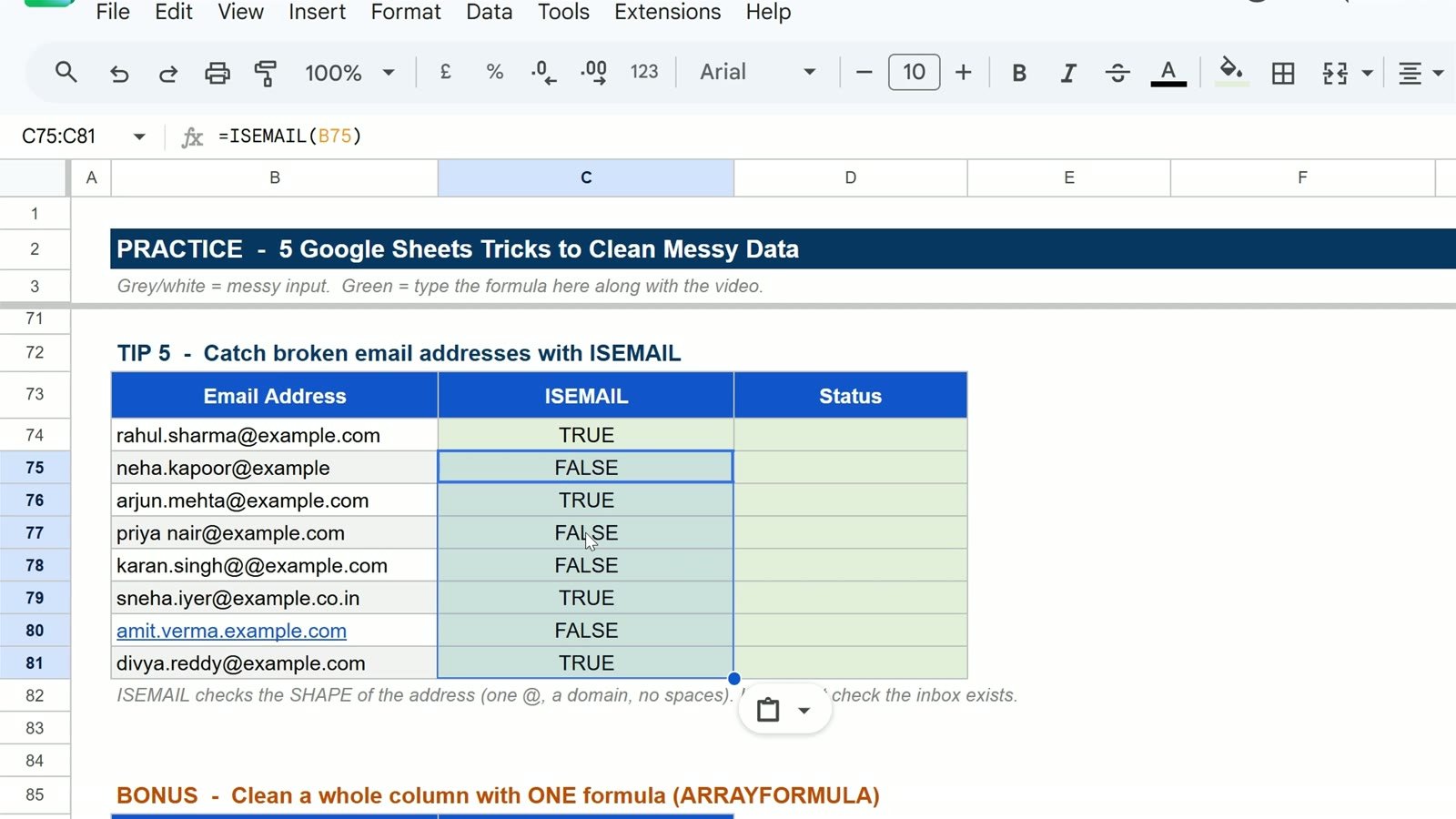
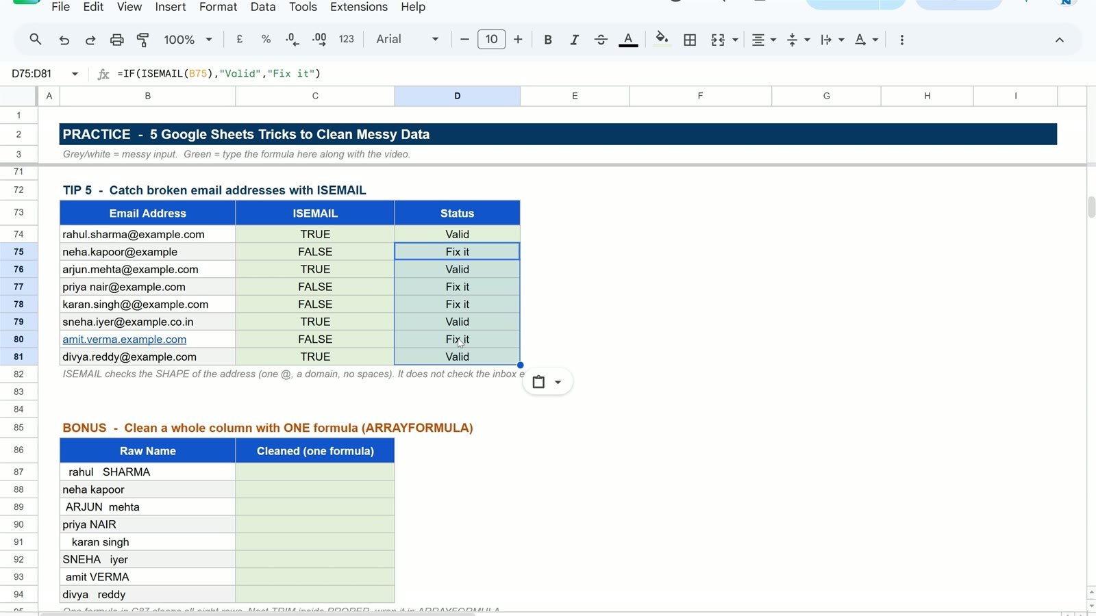
Before you send any email campaign, check the list. Four of these eight addresses are wrong: one has no “.com”, one has a space in the middle, one has two @ signs and one has no @ at all. In C74 type the formula below and copy it down to C81:
=ISEMAIL(B74)Every broken address shows FALSE.
TRUE and FALSE are fine for you, but a team reads words more easily. Wrap ISEMAIL in IF, in D74:
=IF(ISEMAIL(B74),"Valid","Fix it")Copy it down: four addresses to fix. Remember that ISEMAIL checks the format of an address (one @, a domain, no spaces). It does not check whether the inbox really exists.
Bonus: Clean a whole column with ONE formula (ARRAYFORMULA)
So far you wrote one formula and copied it down. The last table has names with both problems, extra spaces and wrong capitals, and you can clean all of them from a single cell. Click C87, type =ARRAYFORMULA(PROPER(TRIM(, then select the whole range B87:B94 and close all three brackets:
=ARRAYFORMULA(PROPER(TRIM(B87:B94)))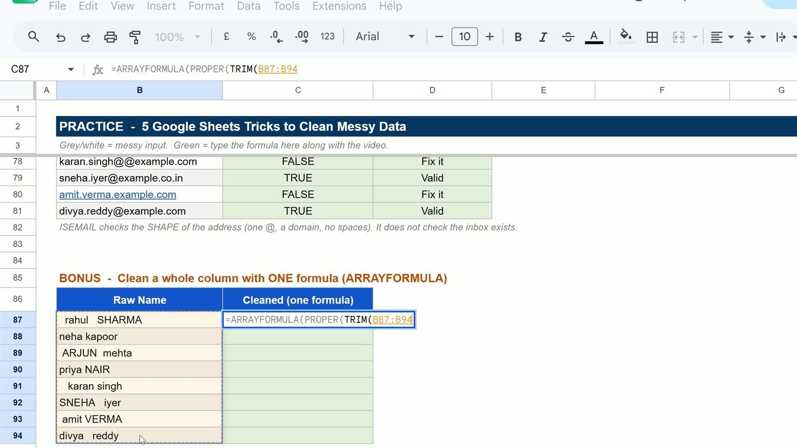
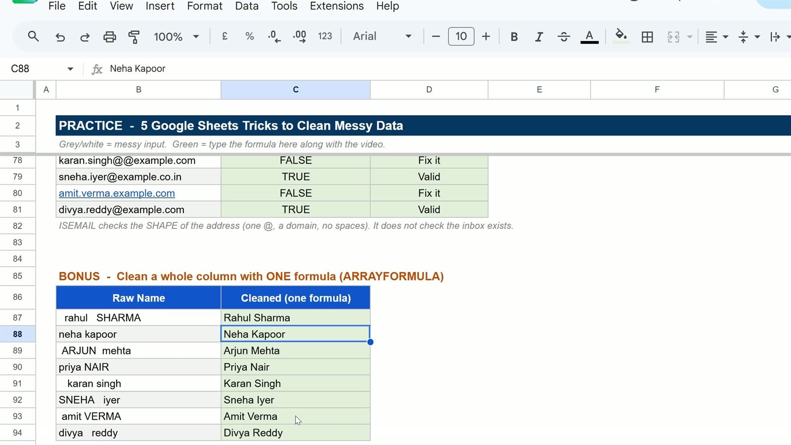
All eight names are cleaned in one shot. TRIM removes the extra spaces, PROPER fixes the capital letters, and ARRAYFORMULA runs both on the whole range, from the one formula in C87.
Formula cheat sheet
| Problem | Formula / menu | Example result |
|---|---|---|
| Extra spaces | =TRIM(B7) |
Length 14 → 12 |
| Hidden line breaks, tabs | =TRIM(CLEAN(B18)) |
Two lines → one line |
| Names in random case | =PROPER(B26) |
rAHUL sHARMA → Rahul Sharma |
| Emails in mixed case | =LOWER(C26) |
all small letters |
| Codes in mixed case | =UPPER(D26) |
INV-2026-101 |
| Full name in one cell | =SPLIT(B37," ") |
Rahul | Sharma |
| “City, State” in one cell | =SPLIT(C37,", ",FALSE) |
Chennai | Tamil Nadu |
| Codes joined with a dash | Data > Split text to columns > Custom “-“ | TSHIRT | M | BLUE |
| Repeated rows (keep the list) | =UNIQUE(B56:D67) |
12 rows → 9 unique |
| Repeated rows (delete them) | Data > Data cleanup > Remove duplicates | 3 removed |
| Broken email addresses | =IF(ISEMAIL(B74),"Valid","Fix it") |
4 to fix |
| A whole column at once | =ARRAYFORMULA(PROPER(TRIM(B87:B94))) |
8 names, 1 formula |
Formula or menu: which should you use?
| Formula (TRIM, SPLIT, UNIQUE…) | Menu (Split text to columns, Remove duplicates, Trim whitespace) | |
|---|---|---|
| Original data | Kept, results go in new cells | Changed in place |
| New or changed data | Updates by itself | Run it again |
| Best for | Lists you refresh every week | A one-time cleanup of an import |
Use formulas when the data keeps coming, and menus when you just need to fix a file once.
Quick tips
- Keep the cells next to SPLIT and UNIQUE empty. They spill into neighbouring cells; if something is in the way you get an error.
- Use LEN to prove the cleanup worked. A length that drops after TRIM is the easiest check.
- Paste values when you need a static clean list. Copy the formula results and use Ctrl + Shift + V.
- Clean before you analyse. Pivot tables, lookups and charts all break on hidden spaces and duplicates. See the XLOOKUP in Google Sheets tutorial for what to do with the clean data next.
More time-savers: 7 Google Sheets hacks that save hours. Keeping an email list? The Newsletter & Email List Growth Tracker pairs well with the ISEMAIL check. The full list of functions is in Google’s Google Sheets function list.
Want to go deeper on formulas like these? The Excel AI Mastery: 100 Formulas course on NextGenTemplates Academy walks you through them with practice files.
Frequently asked questions
What is the difference between TRIM and CLEAN in Google Sheets?
TRIM removes extra spaces: at the start, at the end and repeated spaces between words. CLEAN removes non-printing characters such as line breaks and tabs, which TRIM does not touch. For text pasted from other systems use both: =TRIM(CLEAN(A2)).
Does Google Sheets have a built-in way to remove extra spaces without a formula?
Yes. Select the range and use Data > Data cleanup > Trim whitespace. It changes the cells in place, while TRIM leaves the original and returns a clean copy.
How do I capitalize the first letter of each word in Google Sheets?
Use PROPER, for example =PROPER(B26) turns “rAHUL sHARMA” into “Rahul Sharma”. Use LOWER for all small letters and UPPER for all capitals.
Why does SPLIT break “Tamil Nadu” into two cells?
By default SPLIT treats every character in the delimiter as its own separator, so “, ” splits on the comma and on the space. Add FALSE as the third argument, =SPLIT(C37,", ",FALSE), to treat “, ” as one separator.
What is the difference between UNIQUE and Remove duplicates?
UNIQUE is a formula: it returns the unique rows in new cells and leaves the original list untouched, and it updates when the list changes. Remove duplicates (Data > Data cleanup) deletes the repeated rows from the selected range itself, once.
Does ISEMAIL check if an email address really exists?
No. ISEMAIL only checks that the text is shaped like an email address: one @, a domain and no spaces. A correctly written address with a mailbox that does not exist still returns TRUE.
Can I clean a whole column with one formula?
Yes, with ARRAYFORMULA. For example =ARRAYFORMULA(PROPER(TRIM(B87:B94))) trims and fixes the capitals of eight names from a single cell.
Conclusion
Messy data does not need hours of manual fixing. TRIM and CLEAN handle spaces and hidden characters, PROPER, LOWER and UPPER fix the capitals, SPLIT separates what belongs in different columns, UNIQUE and Remove duplicates get rid of repeated rows, and ISEMAIL catches broken addresses. ARRAYFORMULA then lets you apply the cleanup to a whole column at once. Open the practice file, type each formula yourself, and compare with the Solution sheet. Typing is how these stick.

Written by PK, NeoTech Navigators: step-by-step Google Sheets and Excel tutorials with free practice files.
Download the free practice file
Everything in one page: the view-only Google Sheets link, a one-click Make a copy link, and the full formula cheat sheet from this tutorial.
Free · No sign-up · Opens the Google Sheet in view-only mode, then copy it to your own Drive