Google Sheets is packed with powerful functions that can help you achieve almost anything with your data, from simple calculations to complex conditions. Today, we’re going to dive into two super handy functions—IF and UNICHAR Function—that you can use together to make your data not only more informative but also a little more fun. In this post, I’ll show you how to use these functions to award trophies (or any other symbol) based on students’ performance.
What Are the IF and UNICHAR Functions?
Before we get into the example, let’s first understand what these functions do.
- IF Function: This function allows you to make logical comparisons in your data. Essentially, it checks whether a condition is true or false, and then returns one value if true and another value if false. It’s like having a built-in decision-maker in your spreadsheet.
- UNICHAR Function: This function returns the Unicode character that corresponds to the number you provide. It’s perfect for adding symbols, like a trophy 🏆, directly into your cells.
When you combine these two functions, you can create conditions that automatically add symbols to your data based on specific criteria. Now, let’s see how this works with an example.
Setting Up the Example: Our Data
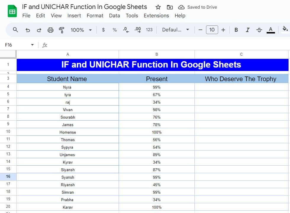
Imagine you’re tracking students’ attendance or performance, and you want to give a visual representation of who deserves a trophy. Here’s what your data might look like:
In this table, you want to award a trophy symbol 🏆 to students who have a “Present” percentage of 85% or higher.
Using IF and UNICHAR Functions: Step-by-Step
Now, let’s use the IF and UNICHAR functions together to automatically assign the trophy symbol to deserving students. Here’s the formula you would use:
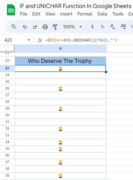
=IF(B4>=85%,UNICHAR(127942),"")
Let’s break down what’s happening in this formula:
- B4>=85%: This part of the formula checks if the student’s percentage is 85% or higher. If it is, the formula returns TRUE; otherwise, it returns FALSE.
- UNICHAR(127942): If the condition is TRUE (the percentage is 85% or higher), this part of the formula inserts the trophy symbol 🏆 into the cell.
“”: If the condition is FALSE (the percentage is lower than 85%), the formula leaves the cell blank.
All you need to do is apply this formula in the “Who Deserves The Trophy” column, and drag it down to apply it to all the students.
The Result: Who Gets the Trophy?
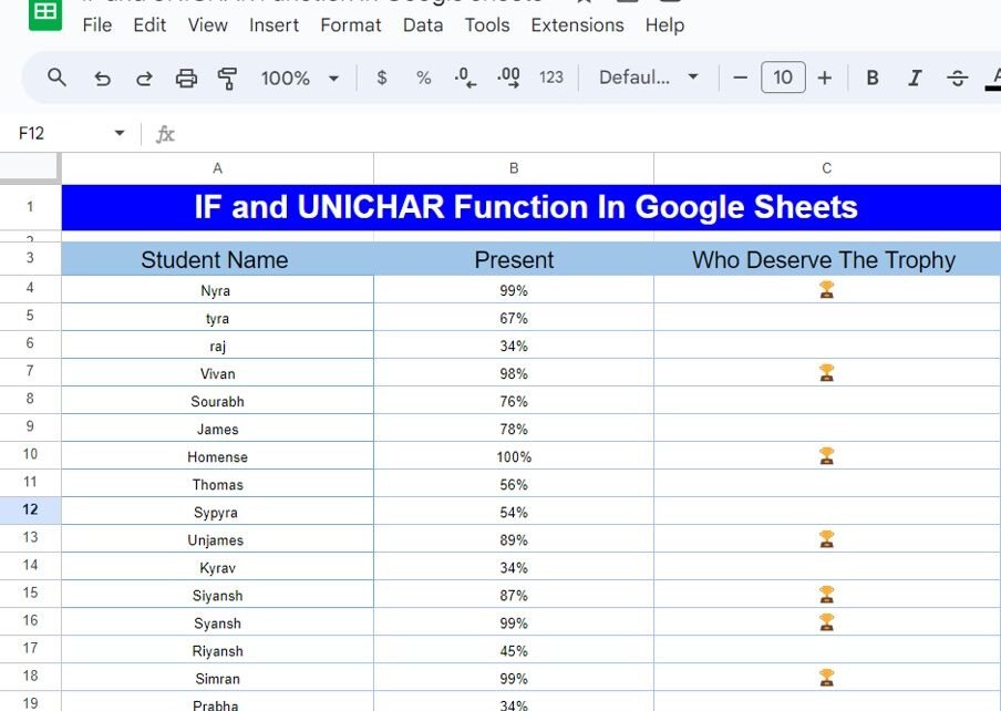
Once you apply the formula, here’s what your table will look like:
As you can see, only the students who have a “Present” percentage of 85% or more have received the trophy symbol. It’s a simple but effective way to visually highlight top performers!
Why You’ll Love Using IF and UNICHAR Together
Combining the IF and UNICHAR functions in Google Sheets is a great way to add a bit of personality and visual appeal to your data. Not only does it make your spreadsheet more engaging, but it also helps you quickly identify key information. Whether you’re working with student performance, sales targets, or any other data, this combination is incredibly versatile and easy to use.
Final Thoughts: Give It a Try!
And there you have it—a quick and fun way to use the IF and UNICHAR functions in Google Sheets! Now that you know how they work, why not try them out in your own projects? You’ll find that adding a little extra flair to your data is both easy and rewarding.
Visit our YouTube channel to learn step-by-step video tutorials
Youtube.com/@NeotechNavigators
View this post on Instagram
Click here to Make the copy of this Template
