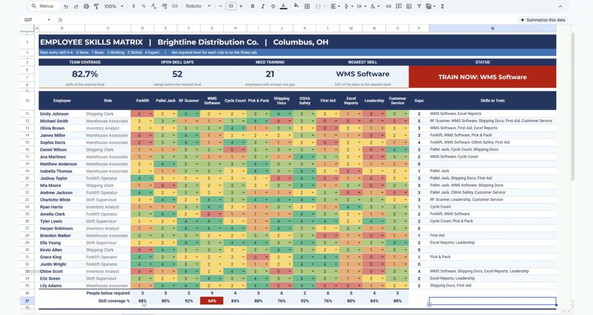
A skills matrix shows who can do what and where the team is exposed. This employee skills matrix in Google Sheets rates 25 employees on 12 skills from 0 to 4, colours the grid as a heatmap, counts each person’s gaps against the level their role needs, lists the skills to train and builds a training plan that sorts itself. In the 15-minute video you build it for Brightline Distribution Co., a made-up distribution center in Columbus, Ohio. Built-in features and formulas only, no add-ons.
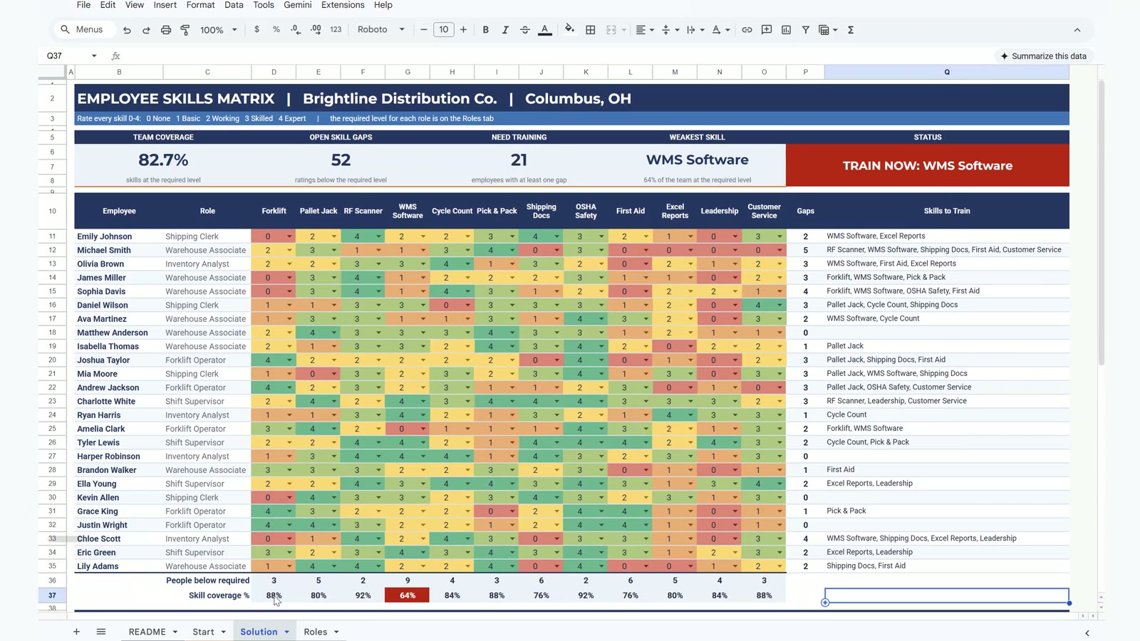
🛒 Get the ready-to-use Employee Skills Matrix Template
Watch the Video Tutorial
Video Overview
The video opens with the finished matrix: team coverage 82.7%, 52 open skill gaps, 21 people who need training, the weakest skill (WMS Software at 64%) and a red TRAIN NOW badge. Then you build it in eight steps: a 0 to 4 rating dropdown, a colour heatmap, gaps per employee, skills to train, gaps and coverage per skill, four KPI cards, the status badge and the training plan. At the end two employees finish their WMS training, coverage rises to 83.3% and the badge turns green.
What You Will Build
- A rating grid with a 0 to 4 dropdown and a red-yellow-green heatmap.
- Gaps per employee measured against the level each role requires.
- Skills to train for every person, written as one readable list.
- Coverage per skill, KPI cards, a status badge and a self-building training plan.

The Start File and the Roles Tab
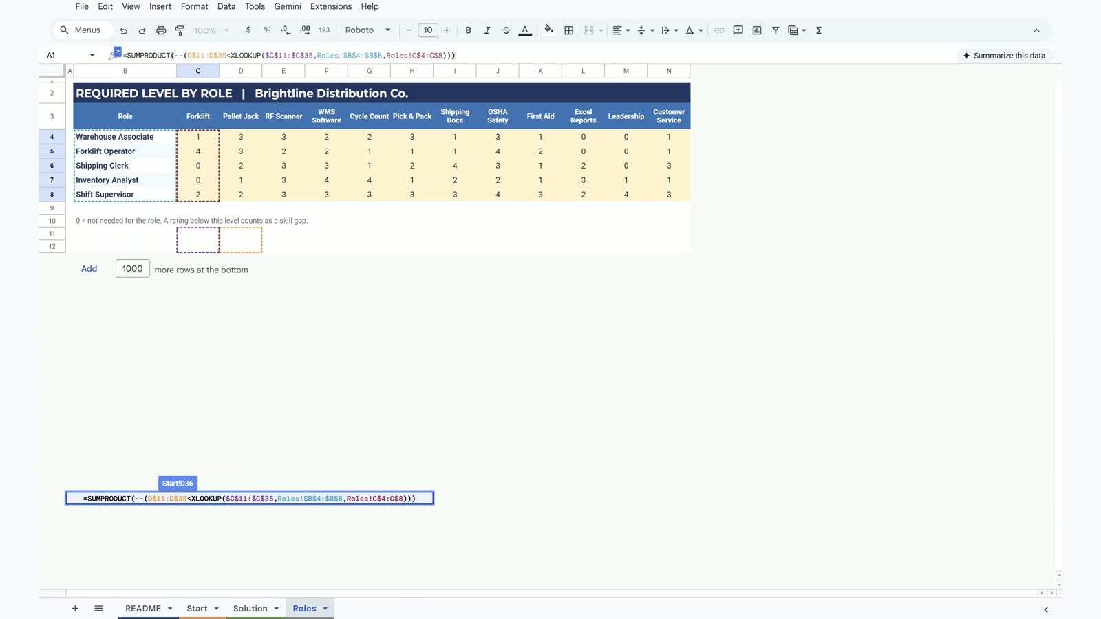
The Start tab holds 25 employees, 5 roles and 12 skills with ratings from 0 (None) to 4 (Expert). The Roles tab lists the required level for each role and skill. The role decides what counts as a gap: a 2 in a skill is fine for a Warehouse Associate but a gap for an Inventory Analyst.
Step 1: 0 to 4 Rating Dropdown
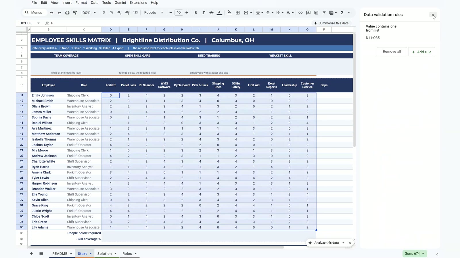
Select the ratings (D11:O35), open Data, then Data validation, and add a dropdown with the items 0, 1, 2, 3 and 4. Set invalid data to Reject the input and keep the display style as plain text so the numbers stay clean on 300 cells.
Step 2: Colour Heatmap
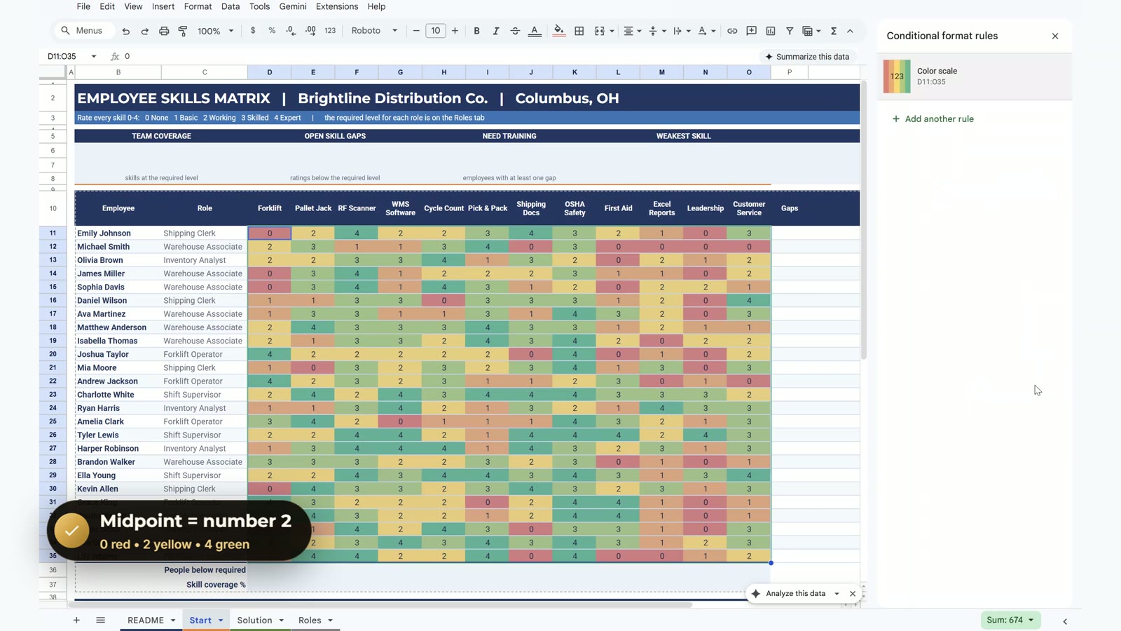
With the same range selected, choose Format, then Conditional formatting, then Color scale. Set the minimum to the number 0 (red), the midpoint to the number 2 (yellow) and the maximum to the number 4 (green). Weak spots now stand out at a glance.
Step 3: Skill Gaps per Employee
In P11 count the skills where the rating is below the role’s required level, then fill down to P35. XLOOKUP returns the whole role row, the comparison gives TRUE or FALSE for each skill, the double minus turns them into 1 and 0, and SUMPRODUCT adds them. Lock the Roles ranges with dollar signs before filling down. Michael Smith, a Warehouse Associate, shows 5 gaps.
=SUMPRODUCT(--(D11:O11<XLOOKUP(C11,Roles!$B$4:$B$8,Roles!$C$4:$N$8)))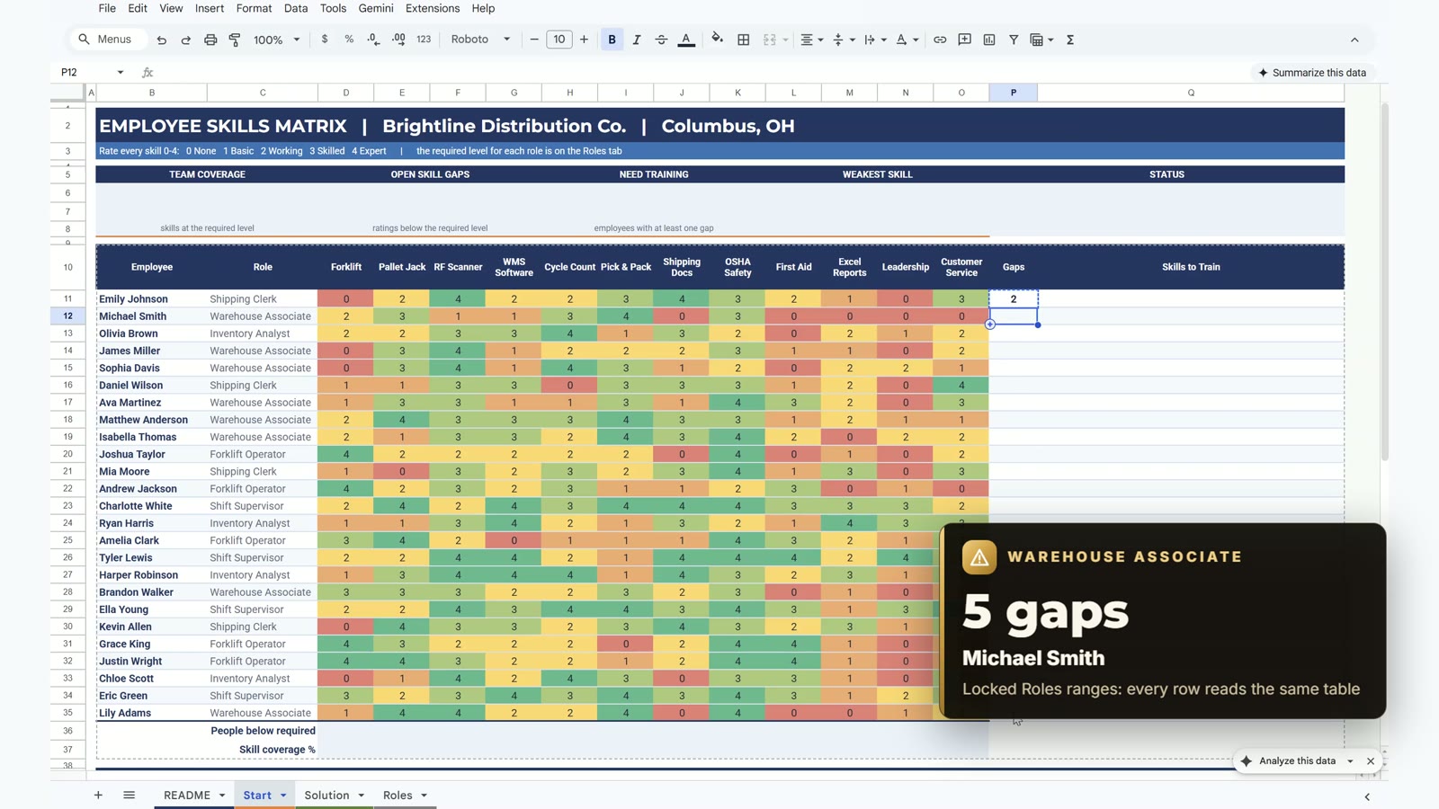
Step 4: Skills to Train
In Q11 write the names of the weak skills as one list. FILTER keeps the skill names whose rating is below the requirement and TEXTJOIN joins them with commas. The IF guard stops the error for people who have no gaps.
=IF(P11=0,"",TEXTJOIN(", ",TRUE,FILTER($D$10:$O$10,D11:O11<XLOOKUP(C11,Roles!$B$4:$B$8,Roles!$C$4:$N$8))))
Step 5: Gaps and Coverage per Skill
Row 36 counts how many people are below the requirement for each skill, and row 37 turns that into coverage. Mixed references are the lesson here: the column moves as you fill right while the rows stay locked. A conditional format turns any coverage under 70% red, and only WMS Software qualifies.
=SUMPRODUCT(--(D$11:D$35<XLOOKUP($C$11:$C$35,Roles!$B$4:$B$8,Roles!C$4:C$8)))=1-D36/COUNTA($B$11:$B$35)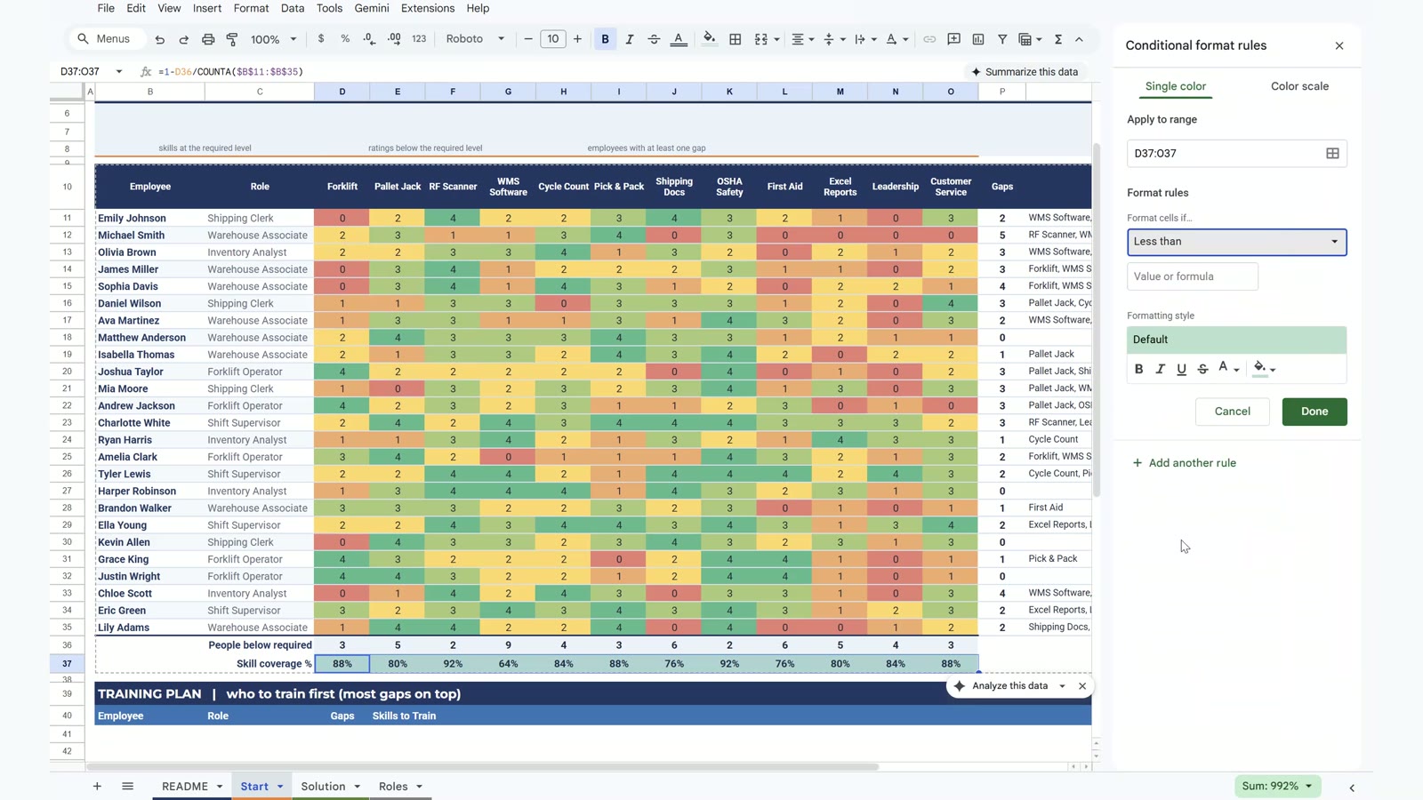
Step 6: KPI Cards
Four cards sit above the grid. Open skill gaps adds the gaps column, team coverage is one minus gaps divided by all ratings, people needing training counts the rows with a gap, and the weakest skill comes from INDEX and MATCH on the lowest coverage.
=SUM(P11:P35)=1-D6/COUNT(D11:O35)=COUNTIF(P11:P35,">0")=INDEX(D10:O10,MATCH(MIN(D37:O37),D37:O37,0))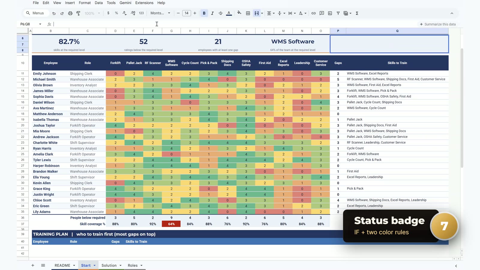
Step 7: Status Badge
One IF turns the weakest coverage into a message, and two conditional formatting rules colour it: green when everything is covered, red when it says TRAIN NOW.
=IF(MIN(D37:O37)>=70%,"ALL SKILLS COVERED","TRAIN NOW: "&L6)
Step 8: Training Plan
One formula builds the plan: FILTER keeps people with at least one gap and SORT puts the biggest gap count first. 21 people appear, Michael Smith first with 5 gaps.
=SORT(FILTER({B11:B35,C11:C35,P11:P35,Q11:Q35},P11:P35>0),3,FALSE)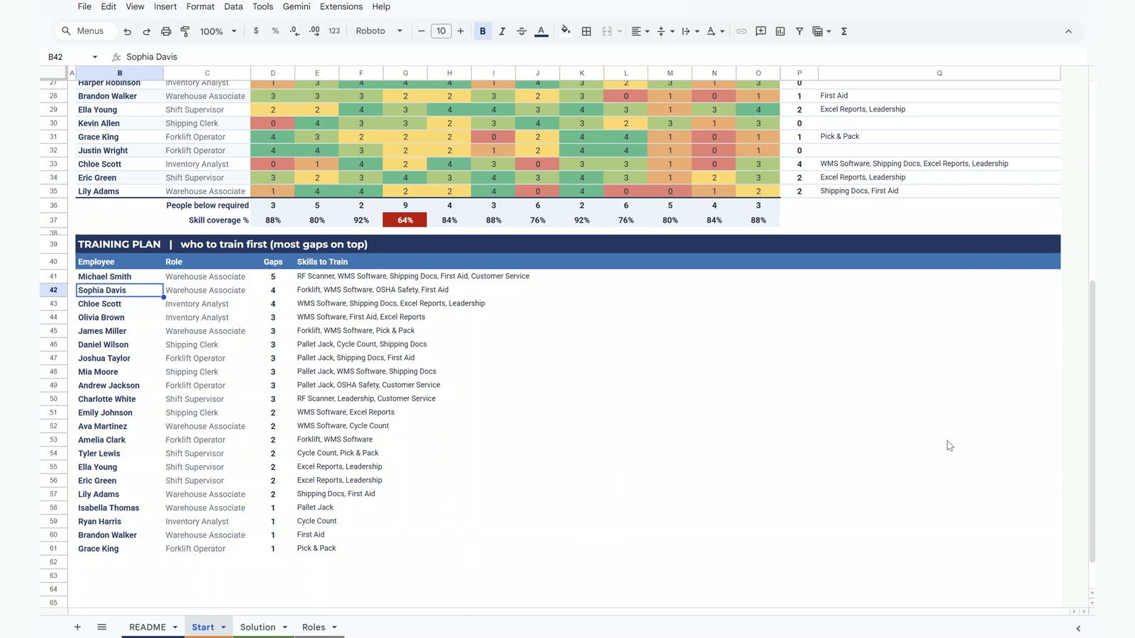
The Payoff: Training Done, Badge Turns Green
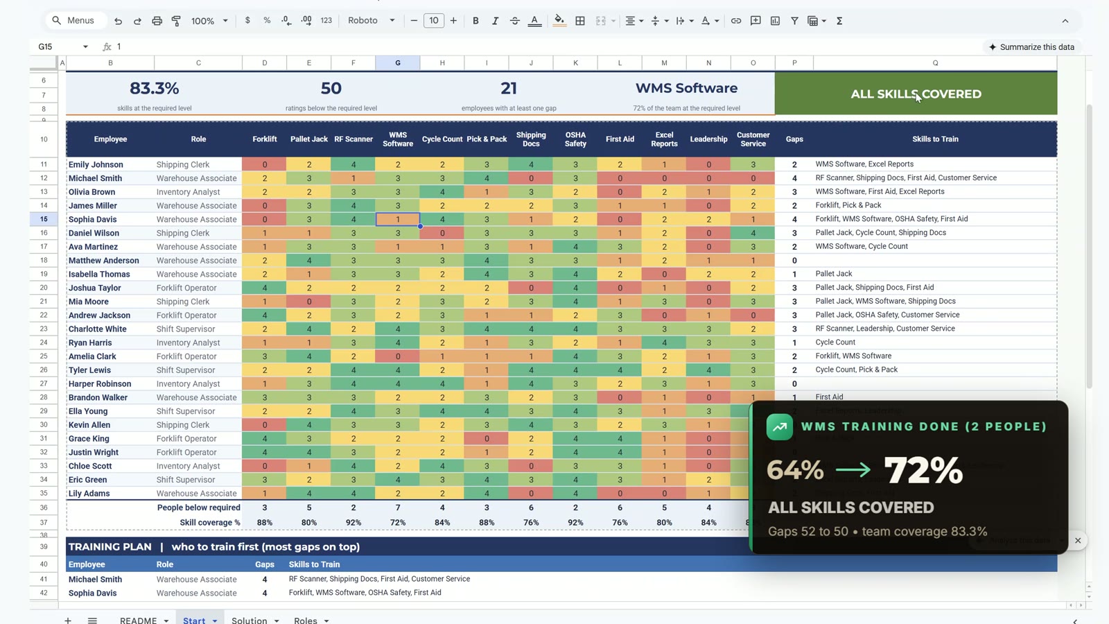
Michael Smith and James Miller finish their WMS training, so you change their ratings from 1 to 3 with the dropdown. WMS coverage rises from 64% to 72%, open gaps fall from 52 to 50, team coverage reaches 83.3% and the badge turns green: ALL SKILLS COVERED.
Want the Ready-to-Use Version?
This is a build-along video. If you would rather skip the building, the Employee Skills Matrix Template in Excel and Google Sheets from Next Gen Templates has all the features ready. To learn Google Sheets step by step, take the Google Sheets Course: Beginner to Advanced.
Frequently Asked Questions
How do I make an employee skills matrix in Google Sheets?
List employees and their roles down the side and skills across the top, rate each cell 0 to 4 with a dropdown, colour the grid with a colour scale, and keep a Roles tab with the level each role needs. Formulas then count gaps per employee, list the skills to train, show coverage per skill and build a training plan. The video builds all of it step by step.
What is a skills gap in this matrix?
A gap is a skill where the employee's rating is below the level their role requires. The role decides: a 2 is fine for a Warehouse Associate but a gap for an Inventory Analyst.
Which formulas does the matrix use?
SUMPRODUCT with XLOOKUP counts gaps per employee, TEXTJOIN with FILTER lists the skills to train, COUNTA, COUNT and COUNTIF drive the coverage and KPI cards, INDEX with MATCH finds the weakest skill, and SORT with FILTER builds the training plan.
Why use XLOOKUP to return a whole row?
XLOOKUP on the Roles tab returns all 12 required levels for the employee's role at once. Comparing the ratings to that row gives 12 TRUE or FALSE values, and SUMPRODUCT adds them up, so one short formula replaces twelve.
How is the status badge decided?
If the lowest skill coverage is 70% or more, the badge says ALL SKILLS COVERED and turns green. Otherwise it says TRAIN NOW followed by the weakest skill, in red.
Do I get the finished template?
The video is a build-along. If you want it ready to use with all features, get the Employee Skills Matrix Template in Excel and Google Sheets from Next Gen Templates.
More Google Sheets tutorials are on the NeoTech Navigators blog and the YouTube playlist. See also the Training Matrix Template in Google Sheets.
More Google Sheets tutorials
- Purchase Order Tracker in Google Sheets: Free Template with Overdue Alerts
- Gantt Chart in Google Sheets: Auto Timeline, Progress Bars & Today Line (Free Template)
- Quote and Estimate Template in Google Sheets: Auto Totals, Tax and PDF (Free Template)
- 10 Google Sheets Formulas for Work: Build One Real Sales Report (Free Practice File)
- Business Expense Tracker in Google Sheets: Free Template with Monthly Summary and Chart
- Asset Tracking System Web App