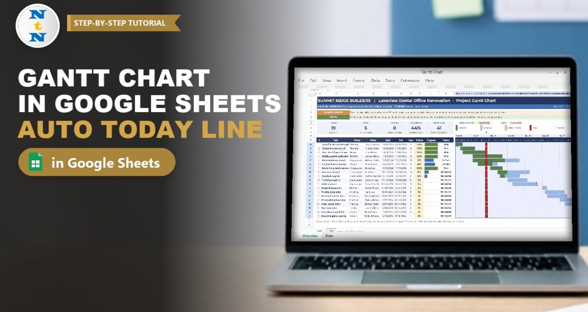
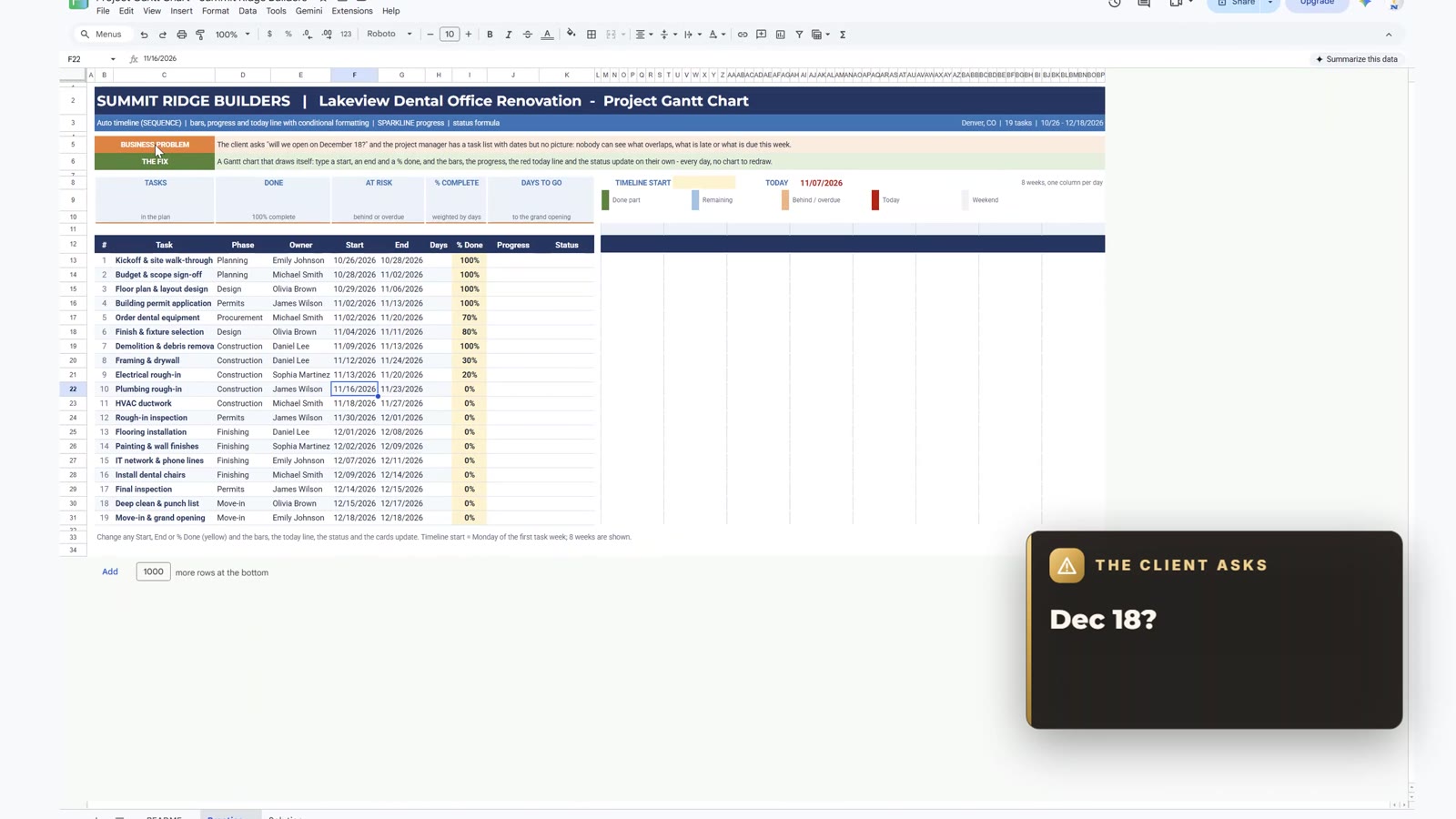
The client asks the same question every week: will we open on December 18? In this tutorial you build a free Gantt chart in Google Sheets for a real office renovation, with an automatic timeline, progress bars, a red today line and a status for every task. You use SEQUENCE, WEEKDAY, SPARKLINE, IF and conditional formatting. Formulas only: no Apps Script, no add-ons.
⬇️ Join Free on Skool & Download the Practice File
Free membership · takes 1 minute · the file is in Classroom → Free Downloads from YouTube
Google Sheets · opens a Make a copy page · Practice + Solution tabs · no add-ons
Watch the Video Tutorial
Video Overview
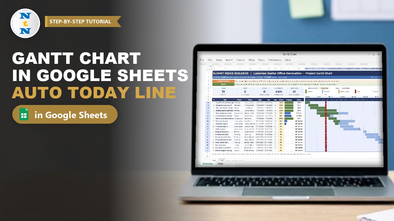
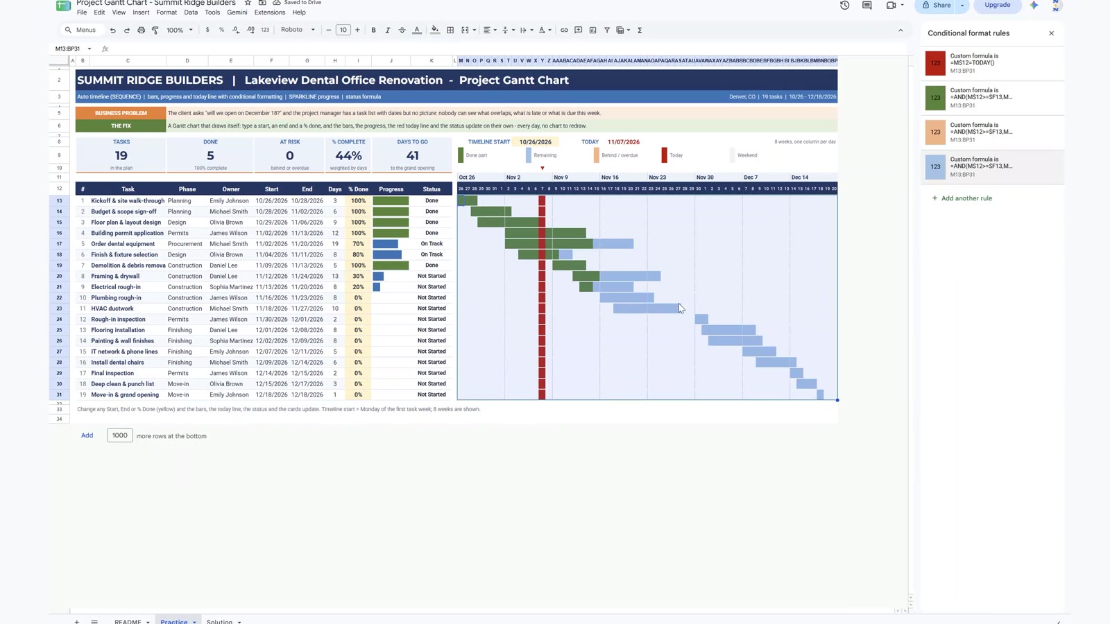
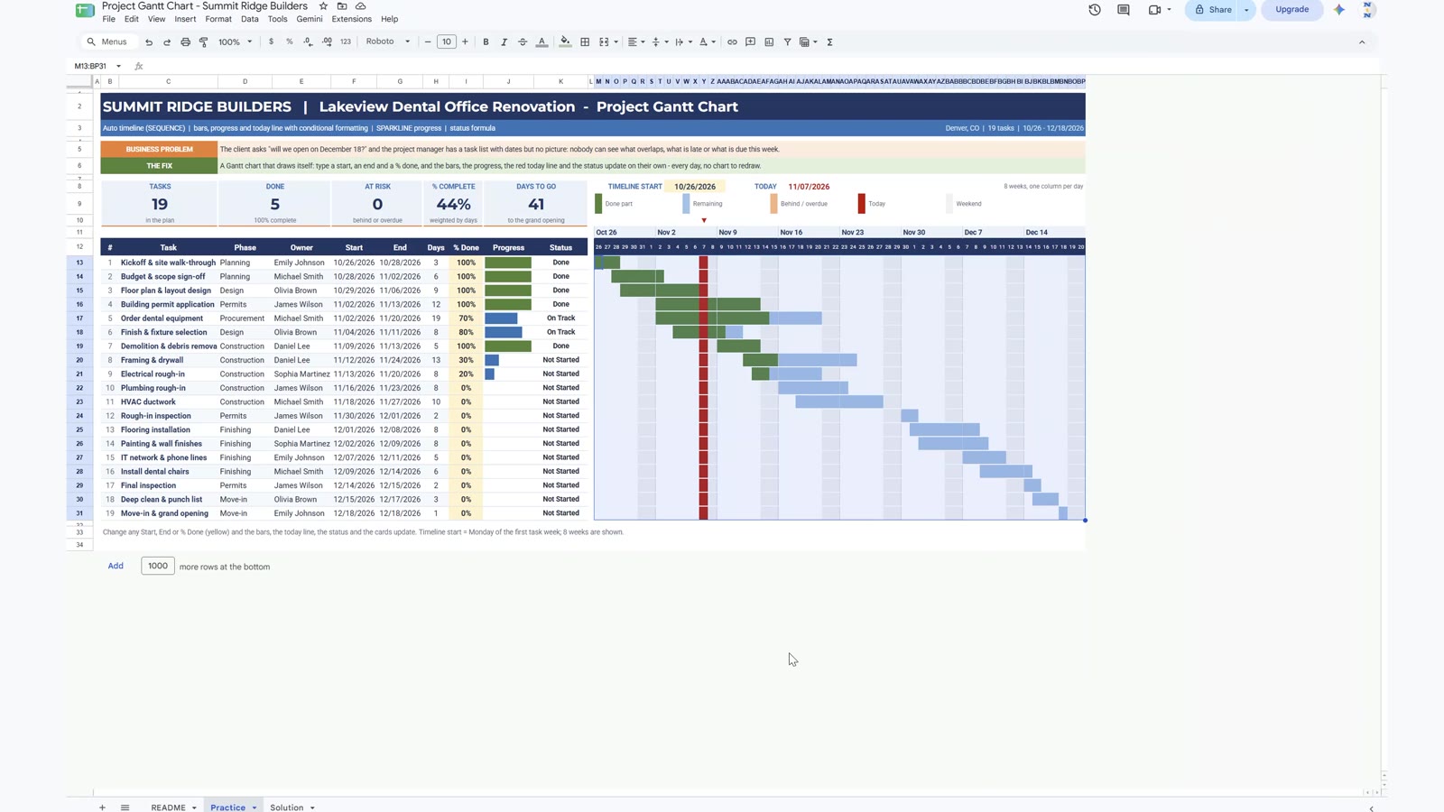
The 15-minute video builds the Gantt chart on the free practice file for the fictional contractor Summit Ridge Builders in Denver, which is turning an empty office into a dental clinic. There are 19 tasks in 7 stages, from October 26 to the grand opening on December 18. Step 1 counts the days of every task. Step 2 finds the Monday where the timeline starts. Step 3 builds 56 dates with one SEQUENCE formula. Step 4 adds SPARKLINE progress bars, step 5 a status formula and step 6 five KPI cards. Step 7 draws the chart with five conditional formatting rules. The payoff changes a percent done and moves a task by a week, and the chart updates by itself.
Gantt Chart in Google Sheets: What You Will Build
- An automatic timeline of 56 days (8 weeks) that starts on the Monday of the first task week.
- Bars for every task from its start date to its end date, with the done part in green.
- A red today line and a small arrow that move one column every day.
- A progress bar in every row with SPARKLINE and a status: Done, On Track, Behind, Overdue or Not Started.
- Five KPI cards: tasks, done, at risk, percent complete and days to go.
- Weekend shading that only shows where there is no bar.
The Practice File
The free file opens a Make a copy page, so you get your own editable Google Sheet. The Practice tab has the 19 tasks with start date, end date and percent done already typed in yellow, and everything else empty. The Solution tab has the finished chart to compare with. The business case: the project manager redraws a chart in slides every week, and by Friday it is out of date. A Gantt chart that draws itself fixes that.
Step 1: Number of Days
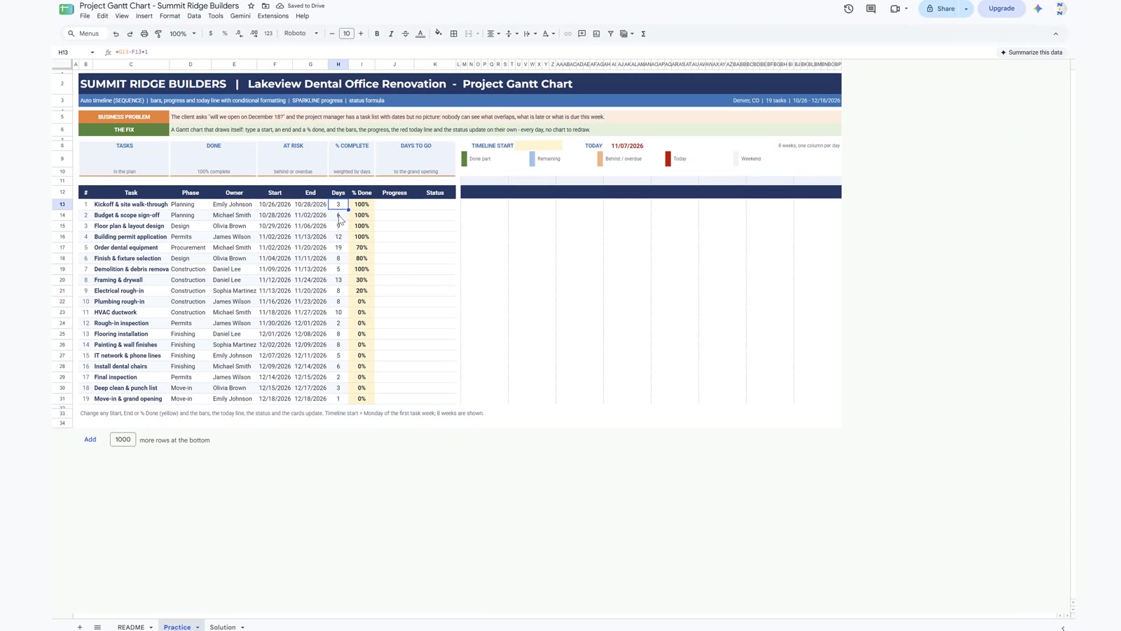
A task that starts on Monday and ends on Wednesday takes three days, not two. In H13 type the end date minus the start date plus one, then double-click the fill handle to copy it down to all 19 tasks:
=G13-F13+1The plus one matters: a task that starts and ends on the same day still takes one day.
Step 2: Timeline Start with MIN and WEEKDAY
The chart should begin on the Monday of the week when the first task starts. In the yellow timeline start cell U8 type:
=MIN(F13:F31)-WEEKDAY(MIN(F13:F31),3)WEEKDAY with type 3 returns 0 for Monday, 1 for Tuesday and so on, so the earliest start date minus its weekday number is always the Monday of that week. Here it gives 10/26/2026. If the first task moved to a Thursday, the cell would still show the Monday before it.
Step 3: Automatic Timeline with SEQUENCE
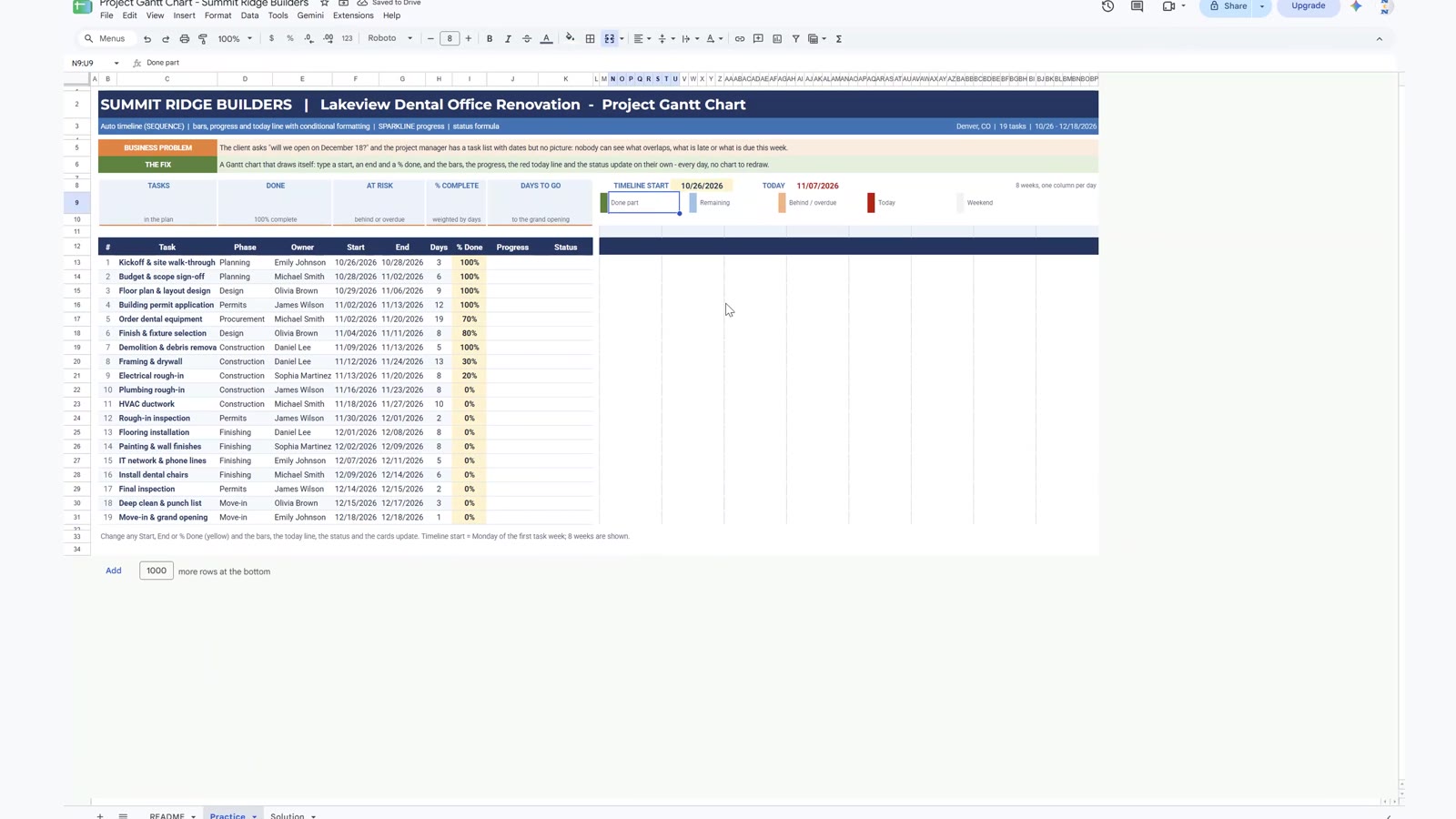
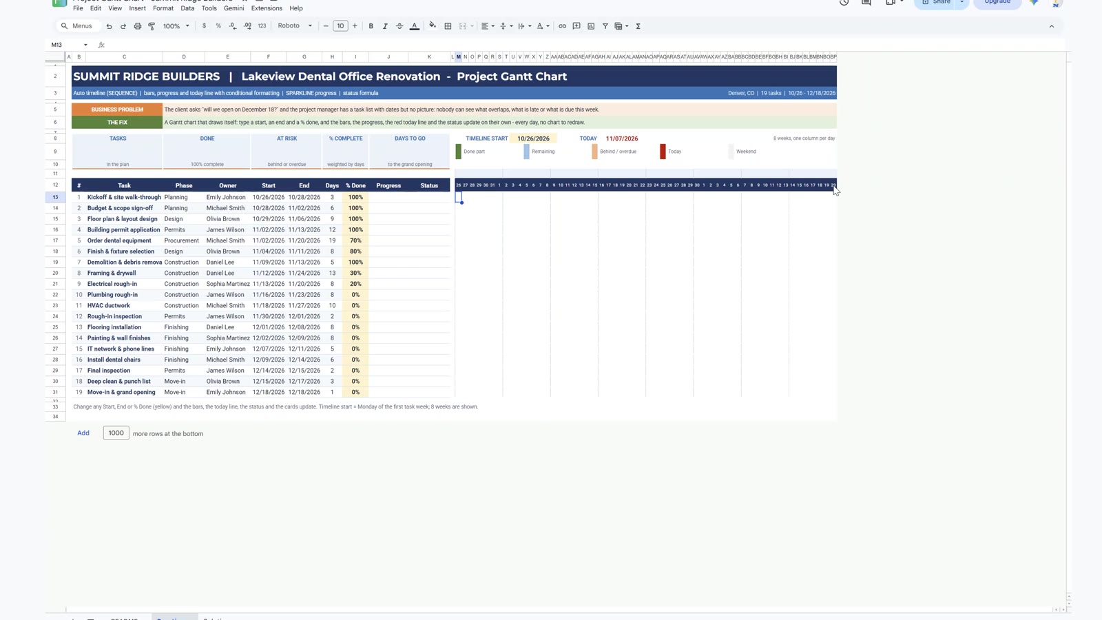
You need 56 dates, one per day for eight weeks, in the dark row above the chart. In M12 type:
=SEQUENCE(1,56,$U$8)Press F4 on the timeline start cell to lock it. One formula gives 56 dates, and the cells are formatted to show only the day number. Trap: SEQUENCE needs the cells to its right to be empty. If anything is typed there you get a #REF! error.
For the week labels in the light row above, type =M12 in M11 (formatted as month and day), then copy it into the first cell of every week. Each copy points to the date right below it:
M11  =M12
(copy M11 into T11, AA11, AH11, AO11, AV11, BC11 and BJ11)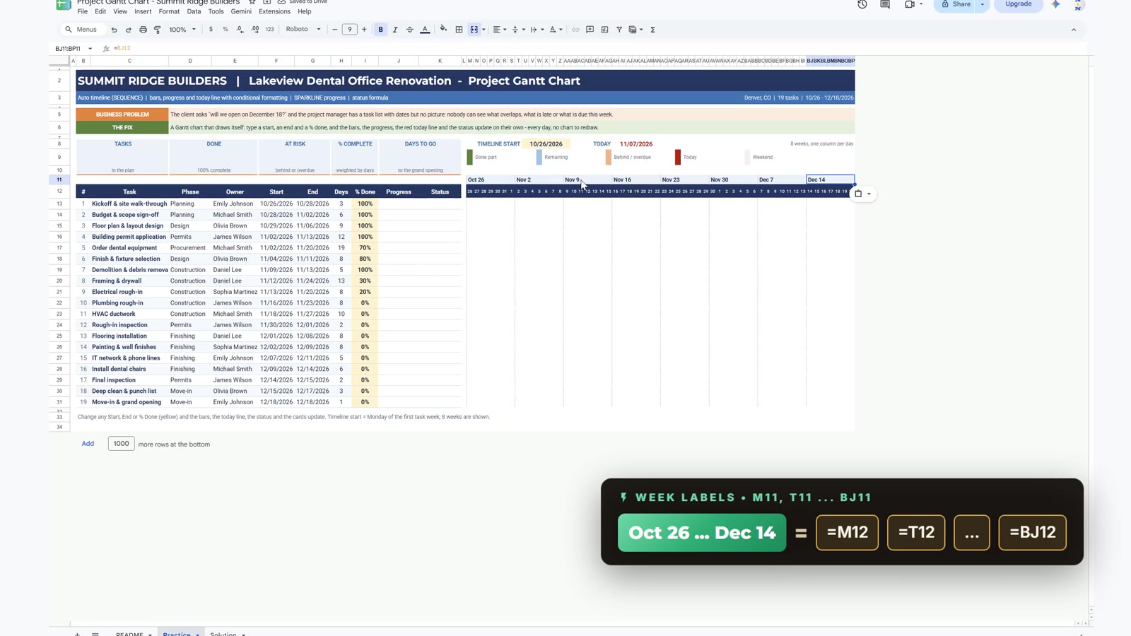
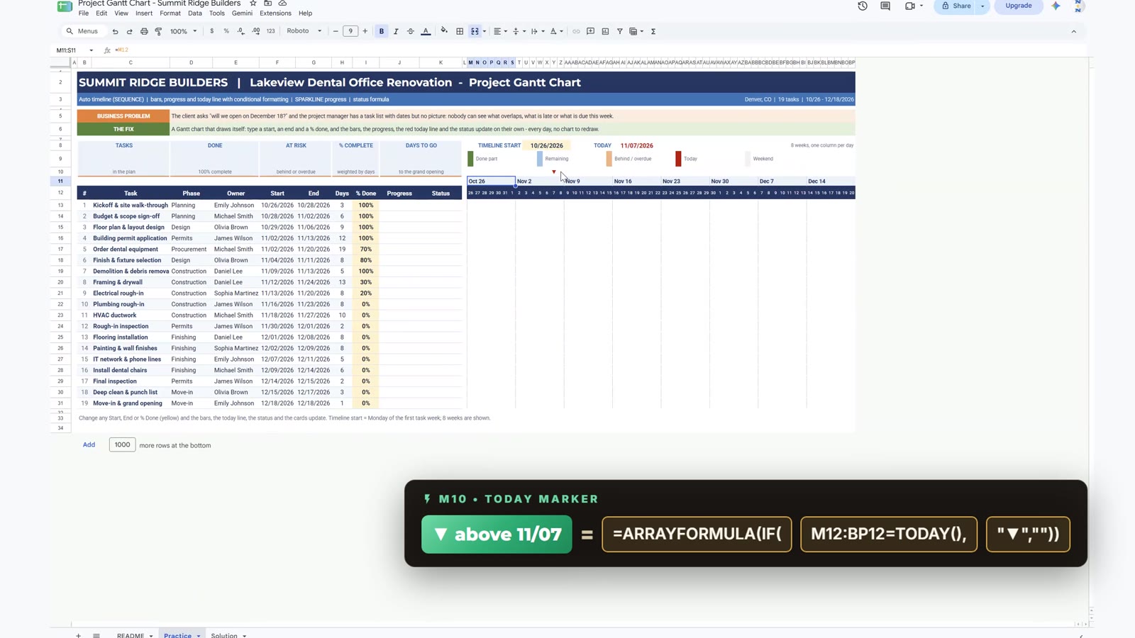
One more header: a small red arrow above today. In M10 type:
=ARRAYFORMULA(IF(M12:BP12=TODAY(),"▼",""))Tomorrow the arrow moves one column to the right on its own, because TODAY changes every day.
Step 4: Progress Bars with SPARKLINE
SPARKLINE draws a tiny chart inside a cell. In J13 type the formula below, then double-click the fill handle. A full green bar means the task is 100 percent done, otherwise the bar is blue, and tasks that have not started have no bar at all:
=SPARKLINE(I13,{"charttype","bar";"max",1;"color1",IF(I13>=1,"#548235","#2E75B6")})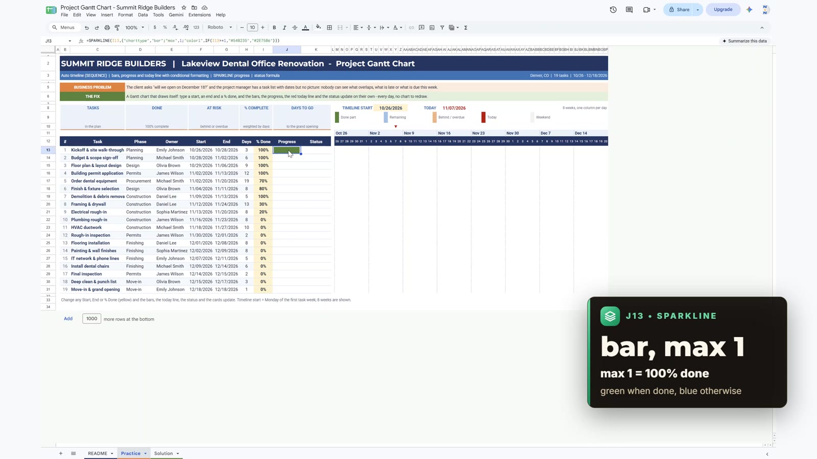
Step 5: The Status Formula
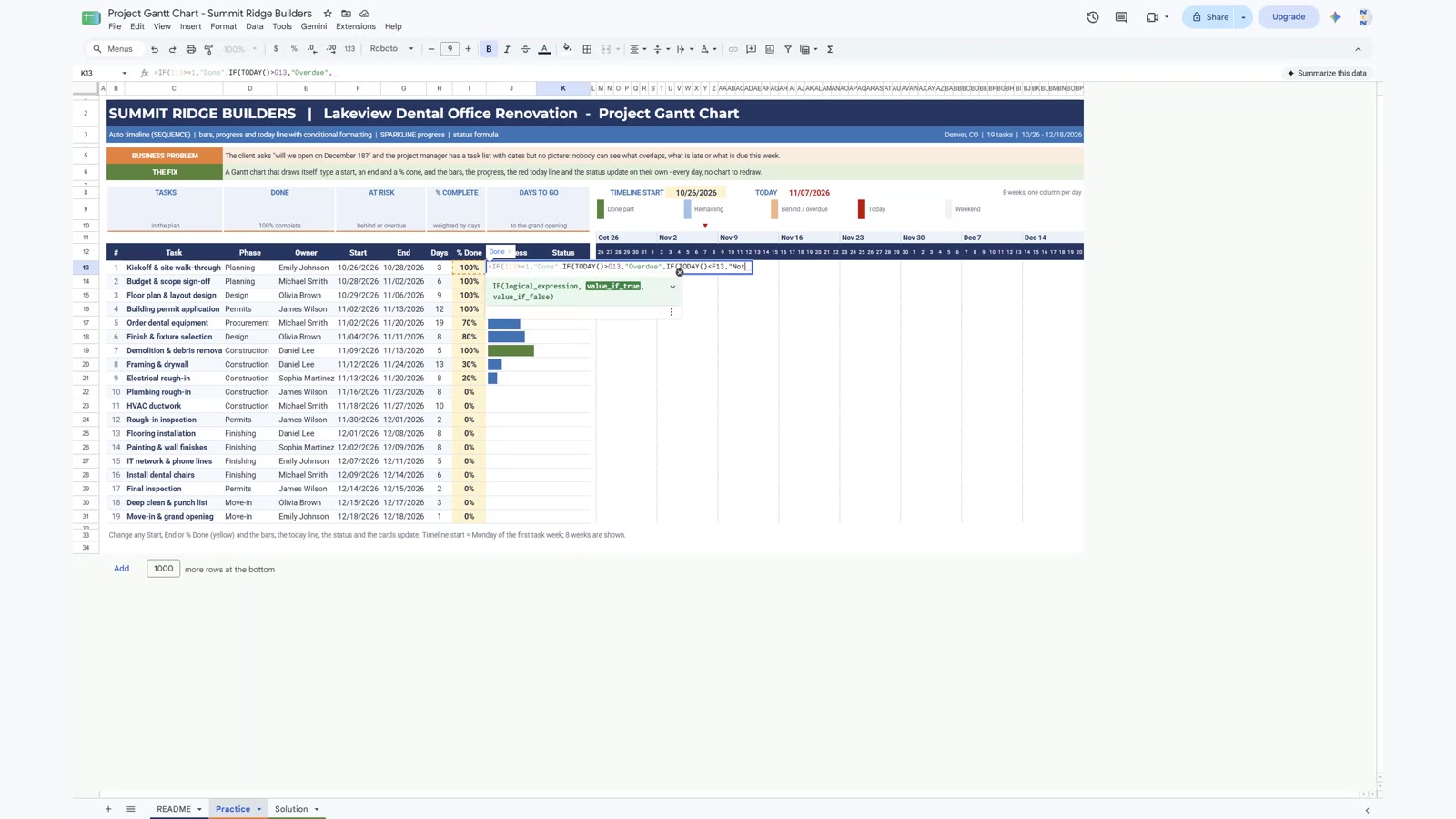
One formula answers the client’s question for every task. It checks four things in this order: 100 percent done is Done, today after the end date is Overdue, today before the start date is Not Started, and for tasks in progress it compares the percent done with where the task should be today. In K13 type:
=IF(I13>=1,"Done",IF(TODAY()>G13,"Overdue",IF(TODAY()<F13,"Not Started",IF(I13+0.1<(TODAY()-F13+1)/H13,"Behind","On Track"))))Where the task should be = (today minus start plus 1) divided by the number of days. If the percent done is more than ten points under that, the task is Behind, otherwise On Track. Fill the formula down to row 31.
Step 6: Five KPI Cards
The cards on top read the table below:
B9  Tasks         =COUNTA(C13:C31)
D9  Done          =COUNTIF(K13:K31,"Done")
F9  At risk       =COUNTIF(K13:K31,"Behind")+COUNTIF(K13:K31,"Overdue")
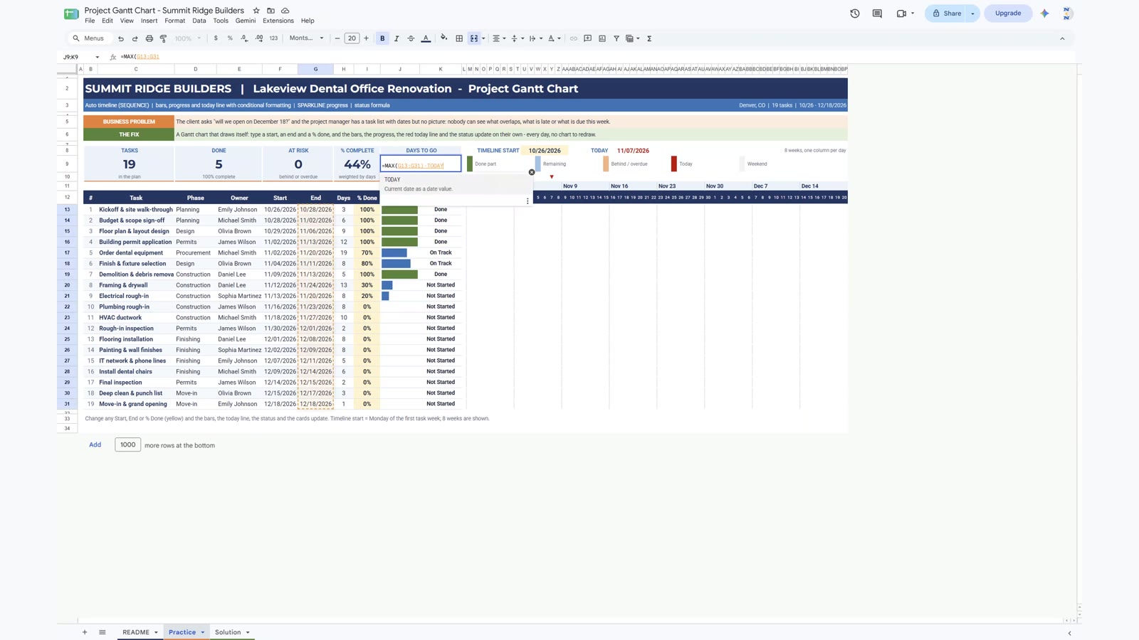
H9  % complete   =SUMPRODUCT(H13:H31,I13:I31)/SUM(H13:H31)
J9  Days to go    =MAX(G13:G31)-TODAY()
On the recording day (November 7, 2026) the cards show 19 tasks, 5 done, 0 at risk, 44% complete and 41 days to go. The percent complete is weighted by days, so a long task counts more than a short one.
Step 7: Draw the Chart with Conditional Formatting
Here is the one rule to remember: when two rules match the same cell, the first rule in the list wins. So add the rules from the most important to the least important: today line, done part, at risk color, normal bar, weekends. Select the chart area M13:BP31, open Format › Conditional formatting, choose Custom formula is and add each rule.
Rule 1: The today line
The formula is written for the top-left cell M13 and then works for every other cell. The dollar sign before 12 locks the date row: the column can change but the row cannot.
=M$12=TODAY() red #C00000, range M13:BP31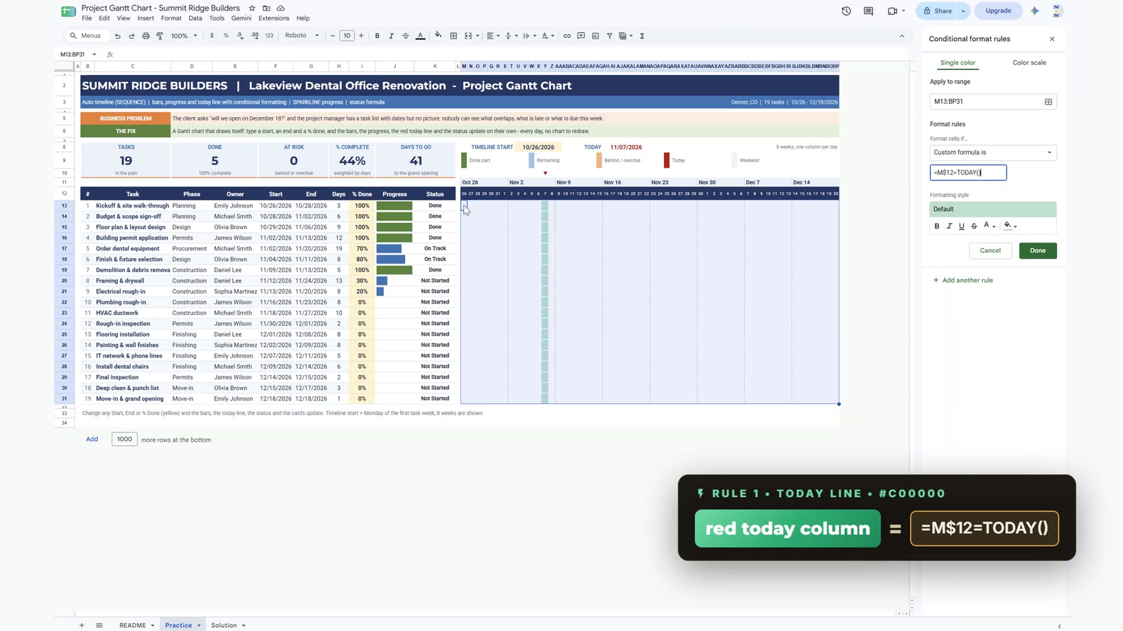
Rule 2: The done part
A cell is green when its date is on or after the start date and before the start date plus the done days (days times percent done, rounded). Here the dollar is before the letter, because every cell must read the start date in column F.
=AND(M$12>=$F13,M$12<$F13+ROUND($H13*$I13)) green #548235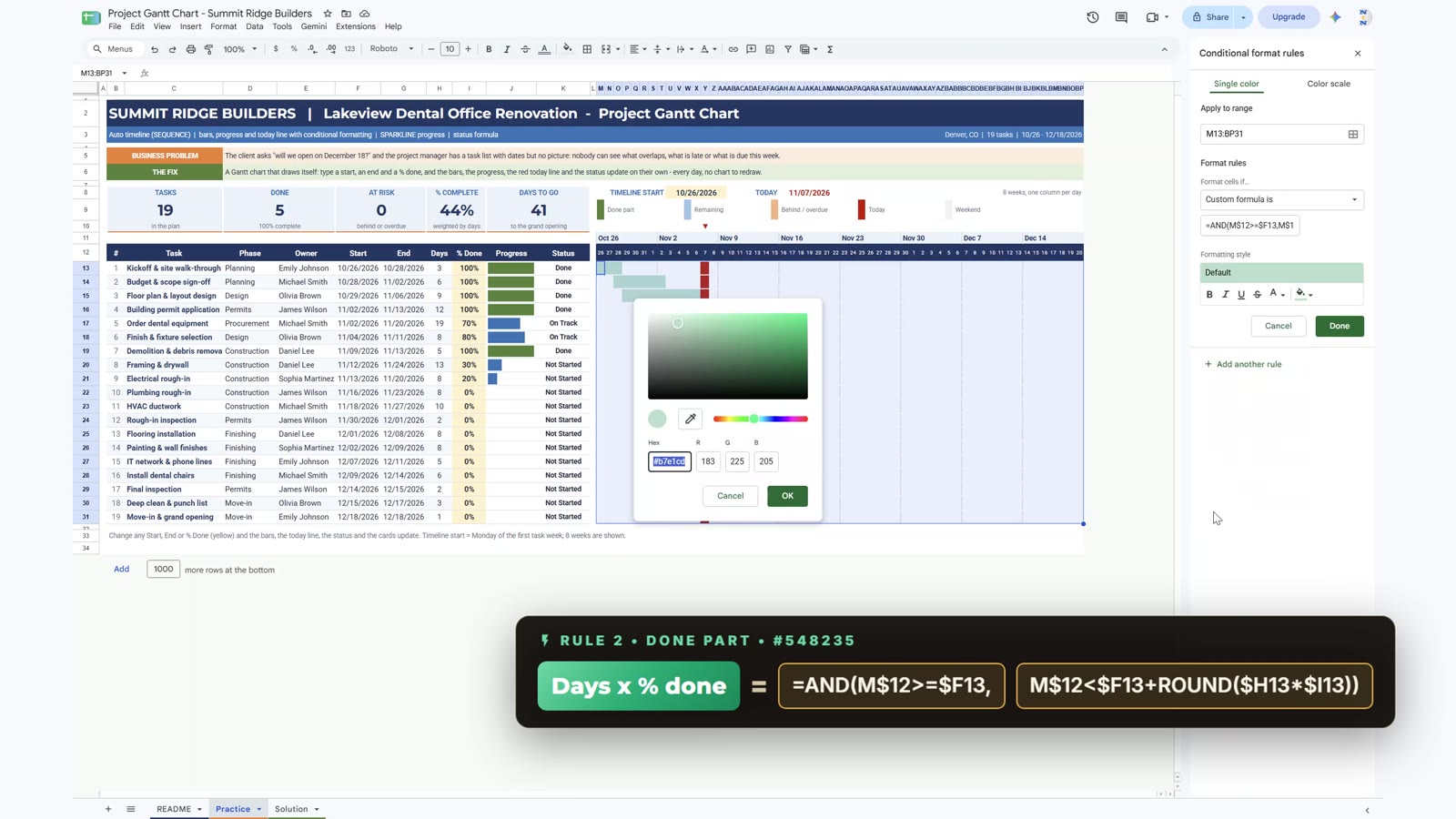
Rules 3 to 5: At risk, normal bar and weekends
=AND(M$12>=$F13,M$12<=$G13,OR($K13="Behind",$K13="Overdue")) orange #F4B183=AND(M$12>=$F13,M$12<=$G13) light blue #9DC3E6=WEEKDAY(M$12,2)>5 light grey #F2F2F2The at risk rule has nothing to colour until a task falls behind, but it is ready for that day. The weekend rule is last, so the grey only shows where no bar is drawn.
The Payoff: Change a Percent and Watch the Chart Update
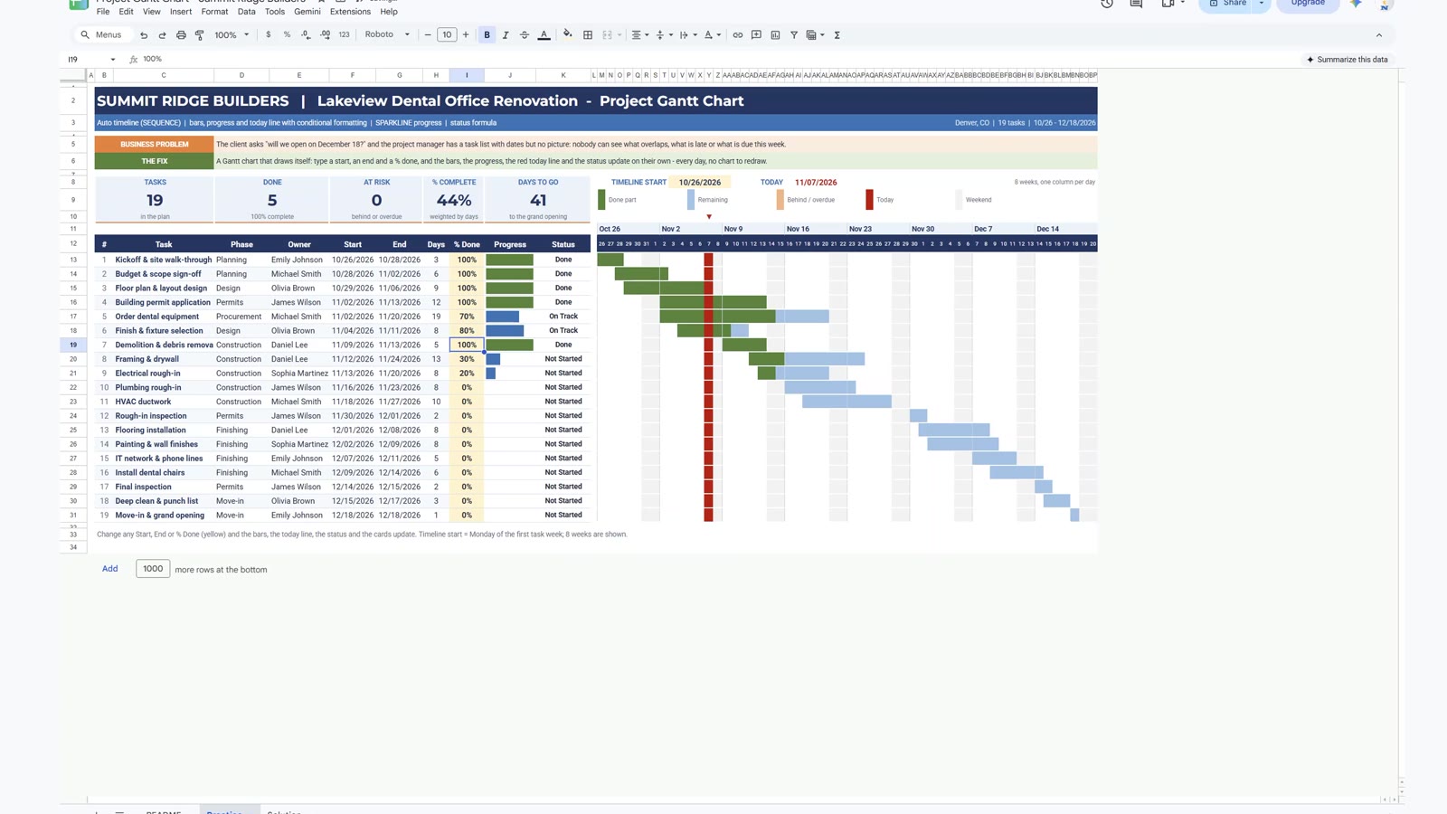
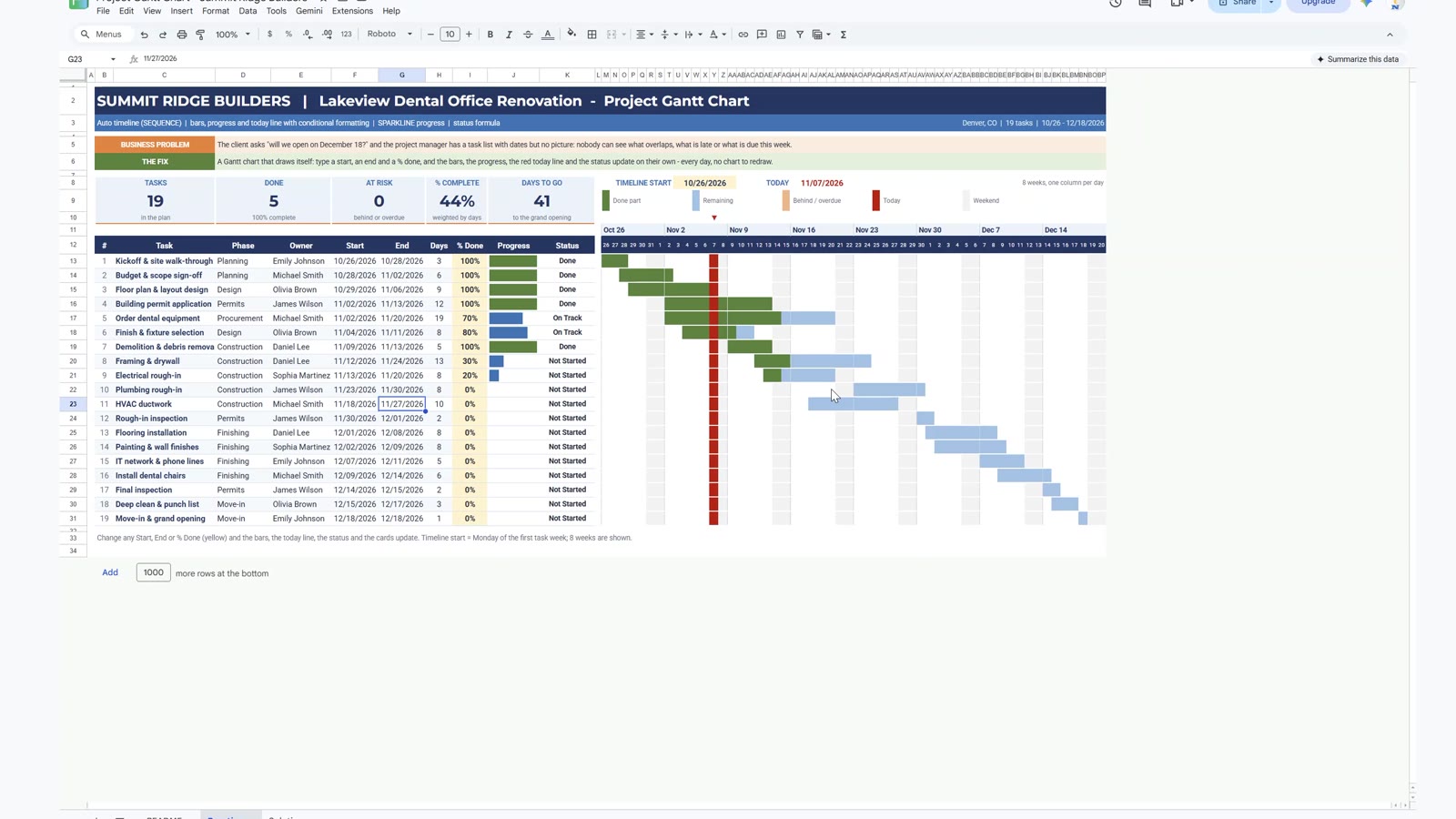
The site manager calls: Finish and fixture selection is only 30 percent done. Type 30% and the status turns Behind, the bar turns orange with a short green part, the at risk card shows 1 and percent complete drops from 44% to 41%. Put it back to 80% and everything is blue and green again. Then move the plumbing work one week later by changing its start to November 23 and its end to November 30: the bar slides one week to the right on its own. No chart to redraw, no shapes to move.
Free Gantt Chart vs the Ready-Made Version
| Need | This free Gantt chart | Project Gantt Chart in Google Sheets |
|---|---|---|
| Auto timeline, bars, progress, today line, status, cards | Yes | Yes |
| Ready-made layout with extra project features | – | Yes |
| Price | Free | Paid |
Tips
- Write every conditional formatting formula for the top-left cell of the range (M13) and let Google Sheets apply it to the rest.
- Check the dollar signs:
M$12locks the date row,$F13locks the start column. - If SEQUENCE shows #REF!, clear the cells to its right.
- Drag the rules in the panel if a color hides another: the first rule in the list wins.
- Each week the team only types the percent done, and everything else updates.
- Google’s SEQUENCE function help page explains the arguments in detail.
Want It Ready-Made?
This free chart is perfect to learn the idea. For a ready-made version with more features see the Project Gantt Chart in Google Sheets on NextGenTemplates.com. To master spreadsheets step by step, the video course Google Sheets Course: Beginner to Advanced on Next Gen Templates Academy teaches it from the basics. More on this site: the project Gantt chart in Google Sheets, the weekly project plan Gantt chart and the marketing KPI dashboard in Google Sheets.
Frequently Asked Questions
How do I make a Gantt chart in Google Sheets?
List the tasks with a start date, an end date and a percent done. Build a row of dates with SEQUENCE, then colour the cells with conditional formatting rules that use a custom formula such as =AND(M$12>=$F13,M$12<=$G13). Google Sheets has no built-in Gantt chart for this, so formulas and rules draw the bars.
Is this Gantt chart template free?
Yes. The practice file opens a Make a copy page in Google Sheets. It has a Practice tab to build along with the video, a Solution tab with the finished chart and a README tab. It uses only formulas and conditional formatting, so no add-ons or Apps Script are needed.
How does the red today line work?
A conditional formatting rule with the custom formula =M$12=TODAY() colours the column whose date in row 12 equals today. TODAY() changes every day, so the line moves by itself. A small ARRAYFORMULA above the dates adds a red arrow.
Why does SEQUENCE show a #REF! error?
SEQUENCE spills its results into the cells to its right. If any of those cells contains something, you get #REF!. Clear the cells M12 to BP12 and enter the formula in M12 only.
Why does the order of the conditional formatting rules matter?
When two rules match the same cell, the first rule in the list wins. Put the rules in this order: today line, done part, at risk color, normal bar, weekends. Then the green done part sits on top of the blue bar and the weekend grey only shows where there is no bar.
What does WEEKDAY with type 3 do?
WEEKDAY(date,3) returns 0 for Monday, 1 for Tuesday and so on up to 6 for Sunday. Subtracting it from the earliest start date always gives the Monday of that week, which is where the timeline should start.
How is the Behind status decided?
A task is Behind when its percent done plus 10 points is still below where it should be today: (today minus start plus 1) divided by the number of days. Done, Overdue and Not Started are checked first, so only tasks in progress can be Behind or On Track.
Download the Practice File
Make your own copy of the practice file and build the Gantt chart along with the video.
⬇️ Join Free on Skool & Download the Practice File
Free membership · takes 1 minute · the file is in Classroom → Free Downloads from YouTube
Google Sheets · opens a Make a copy page · Practice + Solution tabs · no add-ons
About the Author
PK (Priyendra Kumar) runs NeoTech Navigators, PK: An Excel Expert and NextGenTemplates.com, and builds Google Sheets and Excel tools for small businesses. Summit Ridge Builders, Lakeview Dental Group and every name and date in the sample project are fictional.
Conclusion
A Gantt chart in Google Sheets needs no add-ons or scripts. WEEKDAY finds the Monday, SEQUENCE builds the timeline, SPARKLINE draws the progress bars, one IF formula gives the status and five conditional formatting rules in the right order draw the bars, the today line and the weekends. Then you only type the percent done and the whole chart updates by itself.
More Google Sheets tutorials
- Quote and Estimate Template in Google Sheets: Auto Totals, Tax and PDF (Free Template)
- 10 Google Sheets Formulas for Work: Build One Real Sales Report (Free Practice File)
- Business Expense Tracker in Google Sheets: Free Template with Monthly Summary and Chart
- Asset Tracking System Web App
- Task Management Tracker in Google Sheets 2026: Build a Project Task Tracker Step by Step
- Purchase Order and Vendor Management System Web App