The IF and UNICHAR function in Google Sheets work well as a pair: IF makes a yes-or-no decision, and UNICHAR turns a number into a symbol such as a trophy, a tick or a star. Put them together and your sheet can mark top performers with an icon automatically, with no manual typing and no conditional-formatting rules.
This guide is for teachers, team leads and anyone who keeps a score, attendance or target list in Google Sheets. You will work through a real example with 17 students and their attendance percentage, see the exact formula that awards a 🏆 to everyone at 85% or above, and then pick up variations for ticks and crosses, medals, star ratings and counts.
What the IF and UNICHAR Functions Do
IF checks a condition and returns one value when the condition is TRUE and another when it is FALSE. UNICHAR returns the Unicode character for a decimal code number. The trophy emoji 🏆 has the code 127942, so UNICHAR(127942) displays a trophy in the cell.
When UNICHAR sits inside IF, the symbol only appears for rows that pass your test. Everything else can stay blank or show a different symbol.
Syntax
=IF(logical_expression, value_if_true, value_if_false)
=UNICHAR(number)| Argument | Function | What it means |
|---|---|---|
| logical_expression | IF | The test, for example B4>=85%. It must return TRUE or FALSE. |
| value_if_true | IF | What to show when the test is TRUE. Here it is UNICHAR(127942). |
| value_if_false | IF | What to show when the test is FALSE. "" leaves the cell looking empty. |
| number | UNICHAR | The decimal Unicode code point of the character you want, such as 127942 for 🏆. |
The Example Data
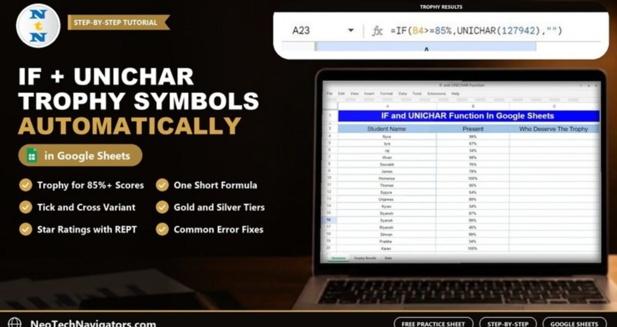
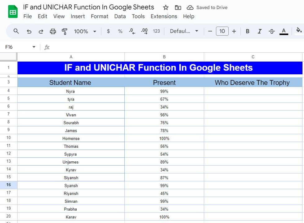
The practice sheet lists 17 students in column A (Student Name) and their attendance in column B (Present), from row 4 to row 20. Column C is headed Who Deserve The Trophy and starts empty. The goal: show a trophy next to every student whose Present value is 85% or higher.
Step-by-Step: Award a Trophy with IF and UNICHAR
- Click the first result cell next to Nyra (row 4).
- Type the formula below and press Enter.
- Select the cell again and drag the small blue fill handle down to row 20, or double-click it.
=IF(B4>=85%,UNICHAR(127942),"")Reading it from left to right:
- B4>=85% asks whether the student’s Present value is at least 85%. Google Sheets stores 85% as 0.85, so this is the same as
B4>=0.85. - UNICHAR(127942) is returned when the answer is TRUE, which shows 🏆.
- “” is returned when the answer is FALSE, so the cell stays blank.
Because B4 has no dollar signs, it moves to B5, B6 and so on as you fill down, so each row checks its own student.
The Result: Who Gets the Trophy
In the practice file the results sit in a separate block (A22:A39) under the same Who Deserve The Trophy heading, with the formula in A23 pointing at B4. You can put the formula in column C instead; the logic is identical.
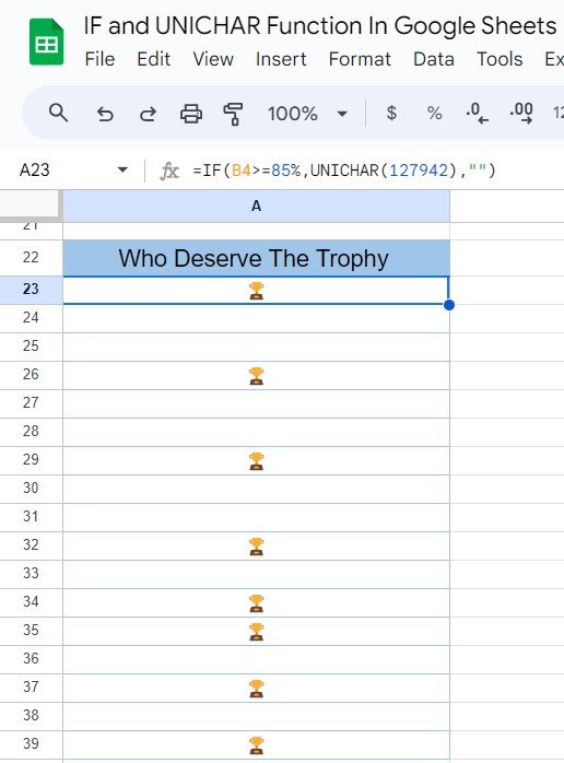 The formula in A23 and the eight trophies it produces.
Eight of the 17 students reach 85% and get a trophy:
| Student | Present | Result |
|---|---|---|
| Nyra | 99% | 🏆 |
| Vivan | 98% | 🏆 |
| Homense | 100% | 🏆 |
| Unjames | 89% | 🏆 |
| Siyansh | 87% | 🏆 |
| Syansh | 99% | 🏆 |
| Simran | 99% | 🏆 |
| Karav | 100% | 🏆 |
Everyone else, from James at 78% down to raj, Kyrav and Prabha at 34%, gets a blank cell.
Useful UNICHAR Codes
Swap 127942 for any of these codes to change the symbol. If you know the symbol but not its number, =UNICODE("🏆") returns 127942, so you can look up any character the same way.
| Code | Symbol | Typical use |
|---|---|---|
| 127942 | 🏆 | Top performer |
| 129351 / 129352 / 129353 | 🥇 🥈 🥉 | First, second, third tier |
| 9989 | ✅ | Pass, done, approved |
| 10060 | ❌ | Fail, missing, rejected |
| 11088 | ⭐ | Ratings |
| 9650 / 9660 | ▲ ▼ | Up or down against a target |
| 128994 / 128308 | 🟢 🔴 | Simple status lights |
Practical Variations
1. Tick or cross for pass and fail
Show a symbol in both cases instead of leaving failures blank. With a 75% pass mark, 10 students get ✅ and 7 get ❌ in the practice data:
=IF(B4>=75%,UNICHAR(9989),UNICHAR(10060))2. Gold and silver tiers with nested IF
Give 🥇 to 95% and above and 🥈 to 85%–94%. Nyra, Vivan, Homense, Syansh, Simran and Karav get gold; Unjames and Siyansh get silver:
=IF(B4>=95%,UNICHAR(129351),IF(B4>=85%,UNICHAR(129352),""))Always test the highest threshold first. If you check 85% first, the 95% branch is never reached.
3. Star rating with REPT
Repeat a star in proportion to the score. Nyra’s 99% rounds to 5 stars and raj’s 34% to 2 stars:
=REPT(UNICHAR(11088),ROUND(B4*5,0))4. One formula for the whole column
Wrap the logic in ARRAYFORMULA so a single cell fills every row, and new rows inside the range are covered automatically:
=ARRAYFORMULA(IF(B4:B20>=85%,UNICHAR(127942),""))5. Count the trophies
Count the qualifying values directly rather than counting the emoji. This returns 8 for the example:
=COUNTIF(B4:B20,">=85%")Common Errors and How to Fix Them
| Problem | Likely cause | Fix |
|---|---|---|
| No trophies appear at all | The test uses >=85 while the cells hold percentages (0.85, 0.99). |
Write 85% or 0.85 in the formula. |
| Every row shows the same result | The reference was locked as $B$4. |
Use a relative B4 so it moves as you fill down. |
| The cell shows an error | The UNICHAR number is not a valid code point (for example 0 or a typo). | Check the code with =UNICODE("symbol"). |
| Results look wrong for some rows | The percentage was typed as text, such as “85 %” with a space. | Re-enter it as a number and apply Format > Number > Percent. |
| The symbol looks different on another device | Emoji are drawn by each system’s font. | Use plain symbols like ✔ (10004) or ▲ when the look must be consistent, such as in printed reports. |
Tips for Using Symbols in Reports
- Keep the threshold in its own cell (for example F2 = 85%) and write
=IF(B4>=$F$2,UNICHAR(127942),""). Changing the target then updates every row. - Symbols are text, so you cannot sum them. Keep calculations on the numbers and use symbols only for display.
- Use one meaning per symbol across a workbook so readers learn it once.
- Pair symbols with a short legend at the top of the sheet if the file will be shared.
If you want more ideas with symbols, see how to use the UNICHAR function in Google Sheets and creating a star rating with the REPT function. For more decision logic, read the IF function with real-life examples and assigning grades with IF in Google Sheets.
If you want to go further with structured lessons on formulas like IF, lookups and nested logic, the Excel AI Mastery: 100 Formulas course on NextGenTemplates Academy covers them step by step, and most of the logic carries straight over to Google Sheets.
Frequently Asked Questions
What does UNICHAR(127942) return in Google Sheets?
It returns the trophy emoji 🏆. The number 127942 is the decimal Unicode code point for that character.
How do I find the UNICHAR code for any symbol?
Paste the symbol into a formula like =UNICODE("⭐"). It returns the code (11088 for the star), which you can then use inside UNICHAR.
Can I use IF and UNICHAR with text conditions instead of numbers?
Yes. For example, =IF(C4="Paid",UNICHAR(9989),UNICHAR(10060)) shows a tick for paid rows and a cross for everything else.
Is this better than conditional formatting icons?
It is different. IF and UNICHAR put a real character in the cell, so it copies, prints and exports with the data. Conditional formatting only changes how a cell looks and does not add icons in Google Sheets.
Does the UNICHAR function work in Excel too?
Yes. Excel has UNICHAR and UNICODE with the same codes, so =IF(B4>=85%,UNICHAR(127942),"") works there as well, although emoji appearance depends on the Excel version and font.
Wrapping Up
IF decides who qualifies and UNICHAR shows it at a glance. In the example, one short formula marked the eight students at 85% or above with a trophy, and the same pattern handles ticks and crosses, medal tiers and star ratings. Open the practice sheet, make a copy with File > Make a copy, and try changing the threshold or the symbol code to see the results update.
📅 Last updated: October 2026